Fully developed baroclinic instability of a 3-layer flow
[1]:
import numpy as np
from numpy import pi
from matplotlib import pyplot as plt

import pyqg
from pyqg import diagnostic_tools as tools
Set up
[2]:
L =  1000.e3     # length scale of box    [m]
Ld = 15.e3       # deformation scale      [m]
kd = 1./Ld       # deformation wavenumber [m^-1]
Nx = 64          # number of grid points

H1 = 500.        # layer 1 thickness  [m]
H2 = 1750.       # layer 2
H3 = 1750.       # layer 3

U1 = 0.05          # layer 1 zonal velocity [m/s]
U2 = 0.025         # layer 2
U3 = 0.00          # layer 3

rho1 = 1025.
rho2 = 1025.275
rho3 = 1025.640

rek = 1.e-7       # linear bottom drag coeff.  [s^-1]
f0  = 0.0001236812857687059 # coriolis param [s^-1]
beta = 1.2130692965249345e-11 # planetary vorticity gradient [m^-1 s^-1]

Ti = Ld/(abs(U1))  # estimate of most unstable e-folding time scale [s]
dt = Ti/200.   # time-step [s]
tmax = 500*Ti      # simulation time [s]
[3]:
m = pyqg.LayeredModel(nx=Nx, nz=3, U = [U1,U2,U3],V = [0.,0.,0.],L=L,f=f0,beta=beta,
                         H = [H1,H2,H3], rho=[rho1,rho2,rho3],rek=rek,
                        dt=dt,tmax=tmax, twrite=10000, tavestart=Ti*200)
INFO: Logger initialized
Initial condition
[4]:
sig = 1.e-7
qi = sig*np.vstack([np.random.randn(m.nx,m.ny)[np.newaxis,],
                    np.random.randn(m.nx,m.ny)[np.newaxis,],
                    np.random.randn(m.nx,m.ny)[np.newaxis,]])
m.set_q(qi)
Run the model
[5]:
m.run()
INFO: Step: 10000, Time: 1.50e+07, KE: 2.38e-04, CFL: 0.009
INFO: Step: 20000, Time: 3.00e+07, KE: 3.59e-02, CFL: 0.126
INFO: Step: 30000, Time: 4.50e+07, KE: 1.70e-01, CFL: 0.191
INFO: Step: 40000, Time: 6.00e+07, KE: 3.59e-01, CFL: 0.213
INFO: Step: 50000, Time: 7.50e+07, KE: 1.91e-01, CFL: 0.192
INFO: Step: 60000, Time: 9.00e+07, KE: 2.24e-01, CFL: 0.207
INFO: Step: 70000, Time: 1.05e+08, KE: 5.46e-01, CFL: 0.307
INFO: Step: 80000, Time: 1.20e+08, KE: 4.94e-01, CFL: 0.252
INFO: Step: 90000, Time: 1.35e+08, KE: 5.62e-01, CFL: 0.210
INFO: Step: 100000, Time: 1.50e+08, KE: 2.70e-01, CFL: 0.218
Xarray Dataset
Notice that the conversion to an xarray dataset requires xarray to be installed on your machine. See here for installation instructions: http://xarray.pydata.org/en/stable/getting-started-guide/installing.html#instructions
[6]:
ds = m.to_dataset()
ds
[6]:
<xarray.Dataset>
Dimensions:            (time: 1, lev: 3, y: 64, x: 64, l: 64, k: 33, lev_mid: 2)
Coordinates:
  * time               (time) float64 1.5e+08
  * lev                (lev) int64 1 2 3
  * lev_mid            (lev_mid) float64 1.5 2.5
  * x                  (x) float64 7.812e+03 2.344e+04 ... 9.766e+05 9.922e+05
  * y                  (y) float64 7.812e+03 2.344e+04 ... 9.766e+05 9.922e+05
  * l                  (l) float64 0.0 6.283e-06 ... -1.257e-05 -6.283e-06
  * k                  (k) float64 0.0 6.283e-06 ... 0.0001948 0.0002011
Data variables: (12/34)
    q                  (time, lev, y, x) float64 0.0001383 ... -8.462e-06
    u                  (time, lev, y, x) float64 0.0413 -0.05882 ... -0.1616
    v                  (time, lev, y, x) float64 -0.357 -0.3027 ... -0.1369
    ufull              (time, lev, y, x) float64 0.0913 -0.008824 ... -0.1616
    vfull              (time, lev, y, x) float64 -0.357 -0.3027 ... -0.1369
    qh                 (time, lev, l, k) complex128 (9.956089311189431e-06+0j...
    ...                 ...
    APEgenspec         (time, l, k) float64 0.0 1.724e-08 ... 5.211e-50
    KEspec_modal       (time, lev, l, k) float64 0.0 0.1616 ... 2.567e-41
    PEspec_modal       (time, lev_mid, l, k) float64 0.0 0.02742 ... 9.974e-42
    APEspec            (time, l, k) float64 0.0 0.04085 ... 2.995e-32 1.117e-41
    KEflux_div         (time, l, k) float64 0.0 6.588e-09 ... 1.817e-24 3.27e-29
    APEflux_div        (time, l, k) float64 0.0 -1.748e-08 ... 1.176e-29
Attributes: (12/24)
    pyqg:beta:       1.2130692965249345e-11
    pyqg:delta:      None
    pyqg:dt:         1500.0
    pyqg:filterfac:  23.6
    pyqg:L:          1000000.0
    pyqg:M:          4096
    ...              ...
    pyqg:tc:         100000
    pyqg:tmax:       150000000.0
    pyqg:twrite:     10000
    pyqg:W:          1000000.0
    title:           pyqg: Python Quasigeostrophic Model
reference: https://pyqg.readthedocs.io/en/latest/index.html- time: 1
- lev: 3
- y: 64
- x: 64
- l: 64
- k: 33
- lev_mid: 2
- time(time)float641.5e+08
- long_name :
- model time
- units :
- s
array([1.5e+08])
- lev(lev)int641 2 3
- long_name :
- vertical levels
array([1, 2, 3])
- lev_mid(lev_mid)float641.5 2.5
- long_name :
- vertical level interface
array([1.5, 2.5])
- x(x)float647.812e+03 2.344e+04 ... 9.922e+05
- long_name :
- real space grid points in the x direction
- units :
- grid point
array([ 7812.5, 23437.5, 39062.5, 54687.5, 70312.5, 85937.5, 101562.5, 117187.5, 132812.5, 148437.5, 164062.5, 179687.5, 195312.5, 210937.5, 226562.5, 242187.5, 257812.5, 273437.5, 289062.5, 304687.5, 320312.5, 335937.5, 351562.5, 367187.5, 382812.5, 398437.5, 414062.5, 429687.5, 445312.5, 460937.5, 476562.5, 492187.5, 507812.5, 523437.5, 539062.5, 554687.5, 570312.5, 585937.5, 601562.5, 617187.5, 632812.5, 648437.5, 664062.5, 679687.5, 695312.5, 710937.5, 726562.5, 742187.5, 757812.5, 773437.5, 789062.5, 804687.5, 820312.5, 835937.5, 851562.5, 867187.5, 882812.5, 898437.5, 914062.5, 929687.5, 945312.5, 960937.5, 976562.5, 992187.5]) - y(y)float647.812e+03 2.344e+04 ... 9.922e+05
- long_name :
- real space grid points in the y direction
- units :
- grid point
array([ 7812.5, 23437.5, 39062.5, 54687.5, 70312.5, 85937.5, 101562.5, 117187.5, 132812.5, 148437.5, 164062.5, 179687.5, 195312.5, 210937.5, 226562.5, 242187.5, 257812.5, 273437.5, 289062.5, 304687.5, 320312.5, 335937.5, 351562.5, 367187.5, 382812.5, 398437.5, 414062.5, 429687.5, 445312.5, 460937.5, 476562.5, 492187.5, 507812.5, 523437.5, 539062.5, 554687.5, 570312.5, 585937.5, 601562.5, 617187.5, 632812.5, 648437.5, 664062.5, 679687.5, 695312.5, 710937.5, 726562.5, 742187.5, 757812.5, 773437.5, 789062.5, 804687.5, 820312.5, 835937.5, 851562.5, 867187.5, 882812.5, 898437.5, 914062.5, 929687.5, 945312.5, 960937.5, 976562.5, 992187.5]) - l(l)float640.0 6.283e-06 ... -6.283e-06
- long_name :
- spectal space grid points in the l direction
- units :
- meridional wavenumber
array([ 0.000000e+00, 6.283185e-06, 1.256637e-05, 1.884956e-05, 2.513274e-05, 3.141593e-05, 3.769911e-05, 4.398230e-05, 5.026548e-05, 5.654867e-05, 6.283185e-05, 6.911504e-05, 7.539822e-05, 8.168141e-05, 8.796459e-05, 9.424778e-05, 1.005310e-04, 1.068142e-04, 1.130973e-04, 1.193805e-04, 1.256637e-04, 1.319469e-04, 1.382301e-04, 1.445133e-04, 1.507964e-04, 1.570796e-04, 1.633628e-04, 1.696460e-04, 1.759292e-04, 1.822124e-04, 1.884956e-04, 1.947787e-04, -2.010619e-04, -1.947787e-04, -1.884956e-04, -1.822124e-04, -1.759292e-04, -1.696460e-04, -1.633628e-04, -1.570796e-04, -1.507964e-04, -1.445133e-04, -1.382301e-04, -1.319469e-04, -1.256637e-04, -1.193805e-04, -1.130973e-04, -1.068142e-04, -1.005310e-04, -9.424778e-05, -8.796459e-05, -8.168141e-05, -7.539822e-05, -6.911504e-05, -6.283185e-05, -5.654867e-05, -5.026548e-05, -4.398230e-05, -3.769911e-05, -3.141593e-05, -2.513274e-05, -1.884956e-05, -1.256637e-05, -6.283185e-06]) - k(k)float640.0 6.283e-06 ... 0.0002011
- long_name :
- spectal space grid points in the k direction
- units :
- zonal wavenumber
array([0.000000e+00, 6.283185e-06, 1.256637e-05, 1.884956e-05, 2.513274e-05,
       3.141593e-05, 3.769911e-05, 4.398230e-05, 5.026548e-05, 5.654867e-05,
       6.283185e-05, 6.911504e-05, 7.539822e-05, 8.168141e-05, 8.796459e-05,
       9.424778e-05, 1.005310e-04, 1.068142e-04, 1.130973e-04, 1.193805e-04,
       1.256637e-04, 1.319469e-04, 1.382301e-04, 1.445133e-04, 1.507964e-04,
       1.570796e-04, 1.633628e-04, 1.696460e-04, 1.759292e-04, 1.822124e-04,
       1.884956e-04, 1.947787e-04, 2.010619e-04])
- q(time, lev, y, x)float640.0001383 0.0001531 ... -8.462e-06
- units :
- s^-1
- long_name :
- potential vorticity in real space
array([[[[ 1.38346980e-04, 1.53111435e-04, 1.54358625e-04, ..., 2.85784794e-05, 5.97597167e-05, 1.03073039e-04], [ 1.55526986e-04, 1.53524409e-04, 1.50892647e-04, ..., 8.25769230e-05, 1.23698526e-04, 1.48529939e-04], [ 1.48367526e-04, 1.48205705e-04, 1.45692383e-04, ..., 1.31462197e-04, 1.48099176e-04, 1.50191465e-04], ..., [ 5.19204079e-05, 4.33539874e-05, 4.83763052e-05, ..., 4.77864081e-05, 6.16317812e-05, 6.16767724e-05], [ 3.33338205e-05, 5.56122936e-05, 9.05724656e-05, ..., 5.60070300e-05, 4.76475925e-05, 3.28277906e-05], [ 8.09059461e-05, 1.19277378e-04, 1.43866140e-04, ..., 3.26033695e-05, 2.64745657e-05, 4.31862319e-05]], [[-3.14821604e-06, -3.34691392e-06, -3.22156397e-06, ..., -9.07885590e-07, -1.41760803e-06, -2.31118202e-06], [-3.43804498e-06, -3.22687252e-06, -3.12563266e-06, ..., -1.93103248e-06, -2.77719890e-06, -3.35298787e-06], [-3.30883090e-06, -3.10657612e-06, -2.94249370e-06, ..., -3.23082253e-06, -3.57502854e-06, -3.51541971e-06], ... [-1.09967043e-06, -8.33961033e-07, -1.19503346e-06, ..., 6.64086608e-07, -8.61071587e-07, -1.61226457e-06], [-7.83581410e-07, -1.62385151e-06, -2.69049401e-06, ..., -8.85270582e-07, -1.38981526e-06, -9.49966290e-07], [-2.10269083e-06, -3.13377258e-06, -3.59703201e-06, ..., -1.07142210e-06, -1.02601363e-06, -1.16995754e-06]], [[-2.22922586e-05, -2.51085147e-05, -2.66009485e-05, ..., -4.67433239e-06, -1.15018987e-05, -1.79691287e-05], [-2.41152832e-05, -2.46907691e-05, -2.43284654e-05, ..., -1.41184427e-05, -1.95993344e-05, -2.25040809e-05], [-2.40001476e-05, -2.30415302e-05, -2.22772635e-05, ..., -2.05670633e-05, -2.27250347e-05, -2.36026284e-05], ..., [-3.57858065e-06, -3.97846279e-06, -8.50311529e-06, ..., -1.81871331e-05, -1.42513043e-05, -8.15398434e-06], [-5.97262082e-06, -1.19213155e-05, -1.75003166e-05, ..., -1.26181190e-05, -5.97364665e-06, -3.31086388e-06], [-1.48583133e-05, -2.02847930e-05, -2.36636303e-05, ..., -3.58576749e-06, -3.52490374e-06, -8.46207095e-06]]]]) - u(time, lev, y, x)float640.0413 -0.05882 ... -0.1225 -0.1616
- units :
- m s^-1
- long_name :
- zonal velocity anomaly
array([[[[ 0.041303 , -0.05882397, -0.14417444, ..., -0.03893048, 0.08009587, 0.10676382], [-0.21434096, -0.27255329, -0.31073178, ..., 0.00168405, -0.0239985 , -0.1179842 ], [-0.44955337, -0.46571795, -0.47602383, ..., -0.21873546, -0.32589967, -0.40809609], ..., [-0.01410377, 0.05719979, 0.17679678, ..., 0.00577776, 0.01378183, -0.01427468], [ 0.07562583, 0.19553651, 0.25139978, ..., -0.08365346, -0.09865378, -0.04424568], [ 0.19058157, 0.18033734, 0.101034 , ..., -0.14784369, -0.03707588, 0.10321181]], [[-0.12441311, -0.14451521, -0.17005709, ..., -0.14611402, -0.12220565, -0.11510011], [-0.25620509, -0.27609834, -0.29449047, ..., -0.21504821, -0.21719475, -0.23419056], [-0.39456666, -0.40474374, -0.41073194, ..., -0.33015652, -0.35382216, -0.37732093], ... [ 0.03556206, 0.05626955, 0.08283948, ..., 0.00827399, 0.01370126, 0.0225854 ], [ 0.00337721, 0.02488118, 0.03822425, ..., -0.04400576, -0.03401513, -0.01786722], [-0.03496625, -0.0338044 , -0.04746255, ..., -0.09951442, -0.07464661, -0.05052528]], [[-0.24040205, -0.22504037, -0.21250011, ..., -0.2253834 , -0.25120238, -0.25260016], [-0.30321383, -0.28771521, -0.27835132, ..., -0.3431754 , -0.33567124, -0.31944543], [-0.38748786, -0.3742275 , -0.36915623, ..., -0.42482371, -0.41439939, -0.40208503], ..., [ 0.05780543, 0.01524783, -0.01522518, ..., 0.08699704, 0.09738834, 0.09059418], [-0.07500959, -0.09905042, -0.10214846, ..., 0.0342105 , 0.01357364, -0.03103424], [-0.17617819, -0.17242753, -0.16214874, ..., -0.07308837, -0.1224911 , -0.16160678]]]]) - v(time, lev, y, x)float64-0.357 -0.3027 ... -0.1296 -0.1369
- units :
- m s^-1
- long_name :
- meridional velocity anomaly
array([[[[-0.35695727, -0.3027412 , -0.27233807, ..., -0.22127154, -0.33463249, -0.38214607], [-0.25947697, -0.23236602, -0.21556218, ..., -0.31879766, -0.33522146, -0.30198907], [-0.21094371, -0.20971568, -0.18681966, ..., -0.26903515, -0.23848051, -0.2142148 ], ..., [-0.19903035, -0.25283605, -0.33252204, ..., -0.08358111, -0.14830597, -0.16808342], [-0.29123028, -0.37164571, -0.41181148, ..., -0.07901642, -0.12613017, -0.19524749], [-0.3934971 , -0.39232027, -0.36279303, ..., -0.09270966, -0.20811628, -0.32577982]], [[-0.24485576, -0.24854691, -0.24851126, ..., -0.13912785, -0.19398269, -0.22899958], [-0.22424936, -0.22630952, -0.2244862 , ..., -0.16036632, -0.19656565, -0.21589393], [-0.20652508, -0.21348054, -0.21226952, ..., -0.15273056, -0.17673665, -0.1935862 ], ... [-0.21122701, -0.23503801, -0.26297337, ..., -0.08961803, -0.14186602, -0.1819652 ], [-0.23092939, -0.2587497 , -0.28092298, ..., -0.09512978, -0.15065944, -0.19575631], [-0.24892488, -0.26561068, -0.27375455, ..., -0.10989494, -0.17058242, -0.21804471]], [[-0.15987948, -0.18727619, -0.21052377, ..., -0.07680151, -0.09681561, -0.12844598], [-0.17623852, -0.2020838 , -0.21770841, ..., -0.05741993, -0.10059158, -0.14279443], [-0.19169735, -0.21373071, -0.21953965, ..., -0.06298255, -0.11491794, -0.1576389 ], ..., [-0.21507356, -0.20191583, -0.19891015, ..., -0.13956753, -0.19139942, -0.21661234], [-0.17185204, -0.17488574, -0.19128171, ..., -0.1481871 , -0.17688261, -0.17825497], [-0.15222788, -0.17475455, -0.19995156, ..., -0.1228191 , -0.12958358, -0.1369193 ]]]]) - ufull(time, lev, y, x)float640.0913 -0.008824 ... -0.1616
- units :
- m s^-1
- long_name :
- zonal full velocities in real space
array([[[[ 0.091303 , -0.00882397, -0.09417444, ..., 0.01106952, 0.13009587, 0.15676382], [-0.16434096, -0.22255329, -0.26073178, ..., 0.05168405, 0.0260015 , -0.0679842 ], [-0.39955337, -0.41571795, -0.42602383, ..., -0.16873546, -0.27589967, -0.35809609], ..., [ 0.03589623, 0.10719979, 0.22679678, ..., 0.05577776, 0.06378183, 0.03572532], [ 0.12562583, 0.24553651, 0.30139978, ..., -0.03365346, -0.04865378, 0.00575432], [ 0.24058157, 0.23033734, 0.151034 , ..., -0.09784369, 0.01292412, 0.15321181]], [[-0.09941311, -0.11951521, -0.14505709, ..., -0.12111402, -0.09720565, -0.09010011], [-0.23120509, -0.25109834, -0.26949047, ..., -0.19004821, -0.19219475, -0.20919056], [-0.36956666, -0.37974374, -0.38573194, ..., -0.30515652, -0.32882216, -0.35232093], ... [ 0.06056206, 0.08126955, 0.10783948, ..., 0.03327399, 0.03870126, 0.0475854 ], [ 0.02837721, 0.04988118, 0.06322425, ..., -0.01900576, -0.00901513, 0.00713278], [-0.00996625, -0.0088044 , -0.02246255, ..., -0.07451442, -0.04964661, -0.02552528]], [[-0.24040205, -0.22504037, -0.21250011, ..., -0.2253834 , -0.25120238, -0.25260016], [-0.30321383, -0.28771521, -0.27835132, ..., -0.3431754 , -0.33567124, -0.31944543], [-0.38748786, -0.3742275 , -0.36915623, ..., -0.42482371, -0.41439939, -0.40208503], ..., [ 0.05780543, 0.01524783, -0.01522518, ..., 0.08699704, 0.09738834, 0.09059418], [-0.07500959, -0.09905042, -0.10214846, ..., 0.0342105 , 0.01357364, -0.03103424], [-0.17617819, -0.17242753, -0.16214874, ..., -0.07308837, -0.1224911 , -0.16160678]]]]) - vfull(time, lev, y, x)float64-0.357 -0.3027 ... -0.1296 -0.1369
- units :
- m s^-1
- long_name :
- meridional full velocities in real space
array([[[[-0.35695727, -0.3027412 , -0.27233807, ..., -0.22127154, -0.33463249, -0.38214607], [-0.25947697, -0.23236602, -0.21556218, ..., -0.31879766, -0.33522146, -0.30198907], [-0.21094371, -0.20971568, -0.18681966, ..., -0.26903515, -0.23848051, -0.2142148 ], ..., [-0.19903035, -0.25283605, -0.33252204, ..., -0.08358111, -0.14830597, -0.16808342], [-0.29123028, -0.37164571, -0.41181148, ..., -0.07901642, -0.12613017, -0.19524749], [-0.3934971 , -0.39232027, -0.36279303, ..., -0.09270966, -0.20811628, -0.32577982]], [[-0.24485576, -0.24854691, -0.24851126, ..., -0.13912785, -0.19398269, -0.22899958], [-0.22424936, -0.22630952, -0.2244862 , ..., -0.16036632, -0.19656565, -0.21589393], [-0.20652508, -0.21348054, -0.21226952, ..., -0.15273056, -0.17673665, -0.1935862 ], ... [-0.21122701, -0.23503801, -0.26297337, ..., -0.08961803, -0.14186602, -0.1819652 ], [-0.23092939, -0.2587497 , -0.28092298, ..., -0.09512978, -0.15065944, -0.19575631], [-0.24892488, -0.26561068, -0.27375455, ..., -0.10989494, -0.17058242, -0.21804471]], [[-0.15987948, -0.18727619, -0.21052377, ..., -0.07680151, -0.09681561, -0.12844598], [-0.17623852, -0.2020838 , -0.21770841, ..., -0.05741993, -0.10059158, -0.14279443], [-0.19169735, -0.21373071, -0.21953965, ..., -0.06298255, -0.11491794, -0.1576389 ], ..., [-0.21507356, -0.20191583, -0.19891015, ..., -0.13956753, -0.19139942, -0.21661234], [-0.17185204, -0.17488574, -0.19128171, ..., -0.1481871 , -0.17688261, -0.17825497], [-0.15222788, -0.17475455, -0.19995156, ..., -0.1228191 , -0.12958358, -0.1369193 ]]]]) - qh(time, lev, l, k)complex128(9.956089311189431e-06+0j) ... (...
- units :
- s^-1
- long_name :
- potential vorticity in spectral space
array([[[[ 9.95608931e-06+0.00000000e+00j, -4.32326894e-02-4.27921198e-02j, -1.00421399e-02+6.16019405e-03j, ..., 1.38458920e-12-2.48029048e-13j, 3.93230287e-16+7.62593058e-17j, -7.50357234e-39+2.95576129e-21j], [ 2.37954035e-01+4.60146769e-02j, 4.71180504e-03+4.54586302e-04j, 5.50009274e-03+2.45759024e-02j, ..., 1.75982307e-13+8.14350640e-13j, -7.02914975e-17+1.76033711e-16j, 8.30966237e-22-1.03367972e-21j], [ 3.23110173e-02+4.99472307e-03j, -9.63865591e-03-7.20626758e-03j, 1.20715405e-02+5.66294150e-03j, ..., -9.18743244e-13+1.03968925e-12j, -4.03490659e-16-1.39972897e-16j, -1.46168671e-21-3.50495213e-21j], ..., [ 3.23376276e-03+1.22926115e-02j, ... -9.99431629e-23-5.05643998e-23j], ..., [-3.34407198e-03-3.30350221e-03j, 8.56289178e-04-1.45655471e-03j, -5.81550966e-04-1.08357119e-03j, ..., -9.87207704e-15+2.11194454e-15j, -4.28645708e-18-4.92580498e-18j, 8.00704917e-23+4.83310570e-23j], [-6.14964212e-03+1.25593405e-03j, 4.23293687e-03-2.26290334e-03j, -1.90530127e-03+2.20227866e-03j, ..., 1.85230017e-14-4.86120473e-14j, 8.42549771e-18+8.69134357e-18j, -1.42885937e-22-1.01362064e-22j], [-3.55660402e-02+6.85712269e-03j, -3.56241190e-03+1.13203289e-02j, -1.10376810e-03-2.21576637e-04j, ..., -1.32259270e-14+4.85691992e-14j, -4.35423529e-18+2.96871909e-17j, -4.43777174e-22+1.30032994e-22j]]]]) - uh(time, lev, l, k)complex128(-377.8057880393274+0j) ... (2.5...
- units :
- m s^-1
- long_name :
- zonal velocity anomaly in spectral space
array([[[[-3.77805788e+02+0.00000000e+00j, -2.70076567e+02-9.41934650e+01j, -1.44755687e+02+3.59323069e+01j, ..., -2.63722281e-10-1.08157244e-10j, 8.38508824e-14-3.32305323e-14j, 6.09774061e-19+6.17433753e-19j], [-8.00290483e+02+0.00000000e+00j, -2.99395447e+02-2.25459743e+01j, 4.35642953e+00-2.41254317e+02j, ..., -9.88984902e-11-1.46453680e-10j, 6.48912308e-14-6.74579179e-15j, 6.55370971e-19+4.46049045e-19j], [-1.50764815e+03+0.00000000e+00j, -1.43028584e+02+4.79852786e+01j, 1.26416072e+02-2.72660955e+02j, ..., 4.96061960e-11-1.55446816e-10j, 4.17340137e-14+1.38036293e-14j, 7.25137579e-19+2.73741848e-19j], ..., [ 5.63093264e+02+0.00000000e+00j, ... 2.86244322e-20+4.23759781e-20j], ..., [ 5.16376010e+02+0.00000000e+00j, -1.06224873e+02-1.93796447e+02j, -2.69259489e+01+2.28616370e+02j, ..., -1.89224298e-11+3.10791739e-12j, 4.52220691e-15-2.44939646e-15j, -3.72172813e-21+5.73608872e-20j], [ 1.18862288e+02+0.00000000e+00j, -7.90969430e+01-1.85243767e+02j, -1.69195293e+01+2.18326820e+02j, ..., -1.51580725e-11+5.00995905e-12j, 3.67498412e-15-2.47854291e-15j, 1.38743807e-20+4.71916603e-20j], [-3.36729799e+02+0.00000000e+00j, -7.47650620e+01-1.36164485e+02j, 6.61278308e+00+2.13566627e+02j, ..., -1.06628903e-11+6.29590944e-12j, 3.10059962e-15-2.02574926e-15j, 2.50589254e-20+4.03090610e-20j]]]]) - vh(time, lev, l, k)complex1280j ... (2.2258960601546507e-19+2...
- units :
- m s^-1
- long_name :
- meridional velocity anomaly in spectral space
array([[[[ 0.00000000e+00+0.00000000e+00j, -5.80817096e+02+5.28850119e+02j, 2.95793574e+02+1.66925408e+02j, ..., 3.12406826e-09+1.61955067e-09j, -4.10204922e-13+1.84371442e-13j, 1.44176362e-17+1.27575862e-17j], [ 0.00000000e+00+0.00000000e+00j, -5.86697110e+02+5.57694129e+02j, 2.73764384e+02+1.82898200e+02j, ..., 2.74213591e-09+2.15062951e-09j, -4.69664531e-13-4.36038528e-14j, 1.60923360e-17+1.07766971e-17j], [ 0.00000000e+00+0.00000000e+00j, -5.85370687e+02+5.81264592e+02j, 2.18357602e+02+1.67413454e+02j, ..., 2.29043675e-09+2.21820927e-09j, -4.57327475e-13-2.06352411e-13j, 1.72193027e-17+8.61422686e-18j], ..., [ 0.00000000e+00+0.00000000e+00j, ... 5.84594730e-19+2.50946517e-18j], ..., [ 0.00000000e+00+0.00000000e+00j, -4.22096506e+02+4.38812244e+02j, 1.26661043e+01+1.43779335e+02j, ..., -1.13834495e-10+1.28531638e-10j, 4.70861947e-14-1.22395964e-14j, -7.73696946e-20+2.87018691e-18j], [ 0.00000000e+00+0.00000000e+00j, -4.41247168e+02+4.47717995e+02j, 5.64582584e+01+1.48651216e+02j, ..., -1.01728344e-10+1.79024149e-10j, 3.94462903e-14-2.46635450e-14j, 8.60590403e-20+2.85254888e-18j], [ 0.00000000e+00+0.00000000e+00j, -4.57053329e+02+4.55082903e+02j, 9.89680158e+01+1.49450078e+02j, ..., -8.49293415e-11+2.17102486e-10j, 3.24906985e-14-3.48865551e-14j, 2.22589606e-19+2.78975288e-18j]]]]) - ph(time, lev, l, k)complex1280j ... (1.3885920480162288e-14-4...
- units :
- m^2 s^-1
- long_name :
- streamfunction in spectral space
array([[[[ 0.00000000e+00+0.00000000e+00j, 8.33000202e+07+5.10064301e+07j, 1.06589563e+07+3.05923395e+06j, ..., -3.10460034e-05+1.76030846e-06j, -1.08046274e-08-3.41402514e-09j, 2.28829946e-31-1.02113164e-13j], [-3.25075958e+08-6.58532210e+07j, -7.47919064e+06+1.54389013e+05j, -1.36830223e+06-1.22583001e+07j, ..., 7.17438827e-08-1.79884605e-05j, 2.73708926e-09-5.71504458e-09j, -3.90791370e-16+5.16918933e-15j], [-1.07790749e+07+5.38361013e+05j, 4.88701679e+06+3.75716766e+06j, -3.26128992e+06+1.49309229e+06j, ..., 2.07914153e-05-1.82958820e-05j, 1.00991338e-08+4.11842196e-09j, 2.54618287e-14+9.56287894e-14j], ..., [ 2.55166310e+06-1.04695730e+06j, ... 2.74950524e-15+2.41416456e-16j], ..., [ 3.71112507e+06+1.13212073e+06j, -1.48949905e+06+5.63958417e+06j, 5.85480333e+05-1.57651509e+06j, ..., 6.60180680e-07+2.46173993e-08j, 1.14073239e-10+1.92222565e-10j, -2.94505461e-15-1.36625509e-15j], [-5.34989191e+06-1.39926422e+06j, 3.08157073e+05-1.30385518e+07j, 3.50086868e+06-7.65791855e+06j, ..., -7.10365663e-07+1.51796557e-06j, -2.22033274e-10-2.75979881e-10j, 2.74548513e-15+2.13848579e-15j], [-2.86971457e+08+5.84628818e+07j, 3.07122964e+05+3.23101111e+07j, 4.94264980e+05+4.80874705e+06j, ..., 2.90482290e-08-1.10514865e-06j, 5.69362640e-11-8.23983804e-10j, 1.38859205e-14-4.20452021e-15j]]]]) - dqhdt(time, lev, l, k)complex128(-0-0j) ... (-4.0876124388172813...
- units :
- s^-2
- long_name :
- previous partial derivative of potential vorticity wrt. time in spectral space
array([[[[-0.00000000e+00-0.00000000e+00j, 1.38090053e-07-2.45090198e-07j, -7.88627637e-09-1.54459458e-07j, ..., 6.26178851e-09-7.03325382e-10j, 6.29449831e-09+1.66471275e-09j, -6.21544739e-27+2.63303558e-09j], [-9.04852908e-09+2.69128899e-08j, 6.53669332e-08+1.22514521e-08j, -1.19034337e-07+1.56023975e-08j, ..., 4.00360451e-10+4.09978088e-09j, -1.63081314e-09+3.66653563e-09j, 3.06802619e-10-5.07629472e-10j], [ 4.13086469e-09-5.37672124e-08j, 4.10328928e-08+6.10880445e-09j, 4.46967951e-08-4.77688948e-09j, ..., -6.62041967e-09+6.58083382e-09j, -1.12256002e-08-4.24780454e-09j, -1.90816775e-09-5.89386008e-09j], ..., [ 2.86359040e-08+4.30835174e-09j, ... -1.49250152e-10-2.48761511e-11j], ..., [-3.86940505e-09-8.40568457e-09j, -9.03972769e-09+1.99808196e-08j, 4.98632620e-09-2.24173282e-08j, ..., -1.97806704e-10+8.72708095e-12j, -2.53706482e-10-3.46711642e-10j, 3.87535545e-10+1.93198349e-10j], [ 3.30992487e-09-5.69183250e-09j, 1.87596029e-08-1.60077169e-08j, 5.59047871e-09+6.43229927e-10j, ..., 1.73032032e-10-3.74673942e-10j, 2.25883182e-10+2.46638603e-10j, -1.71972551e-10-1.31314278e-10j], [ 8.05846966e-10+4.76555115e-09j, 1.03344501e-08-7.81035440e-09j, 7.43874904e-10+2.34682966e-08j, ..., -4.10251269e-11+2.32194363e-10j, -4.86155641e-11+5.04845444e-10j, -4.08761244e-10+1.20700578e-10j]]]]) - Ubg(lev)float640.05 0.025 0.0
- units :
- m s^-1
- long_name :
- background zonal velocity
array([0.05 , 0.025, 0. ])
- Qy(lev)float643.027e-10 -8.326e-12 -5.044e-11
- units :
- m^-1 s^-1
- long_name :
- background potential vorticity gradient
array([ 3.02733732e-10, -8.32553612e-12, -5.04425176e-11])
- dqdt(time, lev, y, x)float648.211e-10 4.369e-10 ... -1.523e-10
- units :
- s^-2
- long_name :
- previous partial derivative of potential vorticity wrt. time in real space
array([[[[ 8.21059746e-10, 4.36940426e-10, 5.33408207e-11, ..., 6.91137238e-10, 8.76469807e-10, 8.92141076e-10], [ 1.75071807e-10, -1.14789679e-10, -1.18048056e-11, ..., 1.06340712e-09, 1.35622612e-09, 9.43040697e-10], [-2.64376580e-10, 1.07206222e-11, -2.56954768e-10, ..., 9.90237412e-10, 1.43867397e-11, -4.60367842e-10], ..., [-2.82638928e-10, -5.66042205e-10, 1.36028000e-10, ..., -2.44009548e-10, 2.32241110e-10, 4.84423232e-10], [ 2.50238082e-10, 1.02534999e-09, 1.08083243e-09, ..., 2.57049937e-10, -3.89610837e-10, -7.21728048e-10], [ 1.16818851e-09, 9.52936004e-10, 6.91115306e-10, ..., -4.98831256e-10, 2.27805158e-10, 1.09305209e-09]], [[-1.48077373e-11, 1.14388238e-12, 4.40907252e-12, ..., -7.66532990e-12, -1.79811131e-11, -2.51441361e-11], [-1.43921529e-12, 9.36802766e-13, -2.26794727e-12, ..., -2.63102952e-11, -2.90490403e-11, -1.76292344e-11], [ 8.74799453e-12, 7.58848413e-12, 9.72129191e-12, ..., -2.33339332e-11, -4.57974162e-12, 7.71150951e-12], ... [ 9.03050039e-12, 3.19321187e-12, -1.24858840e-11, ..., -7.87840877e-12, -1.11629067e-11, -3.51405940e-13], [-1.14072122e-11, -2.66449188e-11, -2.86415350e-11, ..., -8.78997104e-12, 1.10781934e-12, 5.82850356e-12], [-2.63149126e-11, -1.77789157e-11, -3.24223662e-12, ..., 2.12167695e-12, 1.06427340e-12, -1.54485517e-11]], [[-1.11847987e-10, -6.74707980e-11, -3.30047338e-11, ..., -1.18216120e-10, -1.85776836e-10, -1.57291272e-10], [-3.49342317e-11, 1.07721421e-11, 4.79705258e-11, ..., -1.78402504e-10, -1.28651859e-10, -6.82736914e-11], [-7.93697373e-12, 4.58232572e-11, -1.30213943e-11, ..., -1.21576009e-10, -5.81304835e-11, -4.00150889e-11], ..., [ 3.28145410e-11, -6.65651779e-11, -1.29711293e-10, ..., -3.10072381e-12, 4.82871775e-11, 7.55418612e-11], [-1.11871166e-10, -1.47644977e-10, -1.36480584e-10, ..., 6.48680636e-11, 6.91554518e-11, -8.06025232e-12], [-1.65464504e-10, -1.41418290e-10, -1.01319117e-10, ..., 5.70630825e-11, -5.69630486e-11, -1.52320610e-10]]]]) - p(time, lev, y, x)float64-1.216e+05 ... -1.029e+05
- units :
- m^2 s^-1
- long_name :
- streamfunction in real space
array([[[[-121554.75270958, -126704.50691079, -131152.64241816, ..., -105593.49644487, -110001.86303669, -115703.44598756], [-120207.4600794 , -124025.74691243, -127527.64965551, ..., -105618.249784 , -110815.13986657, -115831.59510844], [-114972.91603201, -118275.44560719, -121408.93646799, ..., -104183.05070148, -108162.19483021, -111672.27204856], ..., [-116928.42438818, -120419.07846912, -124976.48995466, ..., -109675.53705332, -111608.31172261, -114082.61633544], [-117090.11996203, -122310.59420267, -128491.34075096, ..., -109220.1263531 , -110840.62614486, -113295.78240094], [-119441.42235797, -125652.28554747, -131556.01707313, ..., -107199.37386027, -109528.80308901, -113727.1390795 ]], [[-111370.71566964, -115235.28131731, -119119.37504178, ..., -101689.57114207, -104315.51717355, -107647.18983849], [-108428.8736821 , -111955.21126567, -115480.76204723, ..., -98925.77252422, -101738.97493934, -104979.74863771], [-103331.05094749, -106622.91649042, -109957.88528687, ..., -94714.43361257, -97300.58729943, -100200.04710953], ... [-112457.8449807 , -115943.25171871, -119827.93321849, ..., -105000.8639344 , -106828.87812512, -109372.33326101], [-112743.54064528, -116576.10951258, -120801.27425567, ..., -104742.73661398, -106678.64743316, -109397.72965768], [-112540.94030851, -116575.56381873, -120797.12002035, ..., -103609.03780069, -105814.74069588, -108871.15336395]], [[-101870.98928874, -104587.68759904, -107701.73157397, ..., -96523.4990232 , -97860.57246824, -99612.85911899], [ -97651.37175381, -100618.10267079, -103910.71305809, ..., -92011.29449176, -93236.93187089, -95148.37982723], [ -92270.99793127, -95460.62744344, -98859.47487308, ..., -85991.58389714, -87388.63003384, -89531.54768901], ..., [-107326.46509099, -110582.941234 , -113694.03861879, ..., -98083.62455753, -100699.54745021, -103924.42002521], [-107176.28621131, -109865.55213176, -112714.35889792, ..., -99059.81579189, -101645.9852423 , -104443.62489077], [-105158.17188258, -107704.84431958, -110633.70938772, ..., -98853.42111531, -100836.84217333, -102909.5471078 ]]]]) - Ensspec(time, lev, l, k)float645.908e-18 2.484e-09 ... 1.944e-49
- long_name :
- enstrophy spectrum
- units :
- s^-2
array([[[[5.90823378e-18, 2.48377414e-09, 1.10099289e-10, ..., 6.30072193e-31, 4.58081439e-38, 2.13919835e-47], [1.88822103e-09, 2.77447492e-10, 1.08946799e-10, ..., 6.20427127e-31, 4.97997451e-38, 2.24437498e-47], [1.06975106e-10, 1.03699620e-10, 8.15427283e-11, ..., 4.46674637e-31, 3.98300263e-38, 1.47489995e-47], ..., [4.57271268e-11, 4.94522737e-11, 4.14033503e-11, ..., 2.24982689e-31, 1.65691991e-38, 4.11998463e-48], [1.06975106e-10, 1.05290261e-10, 7.05741257e-11, ..., 5.26839460e-31, 4.01059360e-38, 1.63621147e-47], [1.88822103e-09, 2.53934165e-10, 1.05432923e-10, ..., 5.59662777e-31, 5.58256532e-38, 2.28928354e-47]], [[3.30413329e-18, 1.61607182e-12, 7.01872780e-14, ..., 3.47439952e-34, 2.79905784e-41, 1.22095678e-50], [1.04573645e-12, 2.17863279e-13, 7.90492106e-14, ..., 2.93264583e-34, 1.96036896e-41, 8.06708889e-51], [7.33454380e-14, 6.62951176e-14, 5.06740308e-14, ..., 1.38528507e-34, 9.01137502e-42, 2.71960349e-51], ... [2.69776413e-14, 2.75659007e-14, 2.40740261e-14, ..., 4.49816768e-35, 1.94510089e-42, 4.22137182e-52], [7.33454380e-14, 6.76849134e-14, 4.50350961e-14, ..., 1.46780013e-34, 9.22598566e-42, 2.68762056e-51], [1.04573645e-12, 2.03592983e-13, 7.62244807e-14, ..., 2.84502289e-34, 2.09341344e-41, 8.08536310e-51]], [[2.99145570e-21, 5.87046886e-11, 3.30781811e-12, ..., 6.44861060e-33, 5.05418706e-40, 1.81683285e-49], [3.68187740e-11, 9.05622497e-12, 3.71724111e-12, ..., 5.76710254e-33, 5.23018807e-40, 1.96212263e-49], [3.25918016e-12, 2.92868293e-12, 2.26820157e-12, ..., 3.66781567e-33, 2.86149903e-40, 9.58524037e-50], ..., [1.38033740e-12, 1.40054050e-12, 1.29940228e-12, ..., 1.60729988e-33, 9.19557761e-41, 2.23406943e-50], [3.25918016e-12, 3.19457003e-12, 2.27037741e-12, ..., 3.80141171e-33, 2.45746947e-40, 1.06987045e-49], [3.68187740e-11, 8.68921408e-12, 3.56851151e-12, ..., 5.67997379e-33, 4.59235542e-40, 1.94378914e-49]]]]) - KEspec(time, lev, l, k)float640.0 0.1877 ... 1.071e-32 4.295e-42
- long_name :
- kinetic energy spectrum
- units :
- m^2 s^-2
array([[[[0.00000000e+00, 1.87692391e-01, 4.28494217e-03, ..., 1.04312694e-23, 7.30356618e-31, 3.28402181e-40], [1.79563988e-01, 1.24294288e-02, 3.52441311e-03, ..., 1.02616338e-23, 7.93671572e-31, 3.44642518e-40], [4.68796818e-03, 3.49463370e-03, 2.31695389e-03, ..., 7.38154209e-24, 6.34372873e-31, 2.26214301e-40], ..., [1.55322059e-03, 1.59032938e-03, 1.14723144e-03, ..., 3.71015518e-24, 2.63200234e-31, 6.30294187e-41], [4.68796818e-03, 3.41541673e-03, 2.06739547e-03, ..., 8.70909501e-24, 6.38692219e-31, 2.50996155e-40], [1.79563988e-01, 1.04063433e-02, 3.30124506e-03, ..., 9.25890369e-24, 8.90110341e-31, 3.51626753e-40]], [[0.00000000e+00, 1.67234494e-01, 3.25136572e-03, ..., 6.03162017e-26, 3.86576476e-33, 1.53411303e-42], [1.61968328e-01, 1.04004758e-02, 2.53918601e-03, ..., 5.68257267e-26, 4.03409414e-33, 1.60757389e-42], [3.65586491e-03, 2.46238052e-03, 1.39783253e-03, ..., 4.15203626e-26, 3.29587160e-33, 1.03885693e-42], ... [9.85661391e-04, 9.52727381e-04, 6.00530062e-04, ..., 2.13879737e-26, 1.34789137e-33, 2.88376112e-43], [3.65586491e-03, 2.40612739e-03, 1.29671536e-03, ..., 4.95038076e-26, 3.29995048e-33, 1.16068404e-42], [1.61968328e-01, 8.64600025e-03, 2.35384572e-03, ..., 5.25651352e-26, 4.60349663e-33, 1.66749075e-42]], [[0.00000000e+00, 1.49182766e-01, 2.62668246e-03, ..., 1.59055697e-25, 1.18151137e-32, 4.02510902e-42], [1.46697691e-01, 8.90494723e-03, 2.02390735e-03, ..., 1.41853742e-25, 1.21989180e-32, 4.32066750e-42], [3.06851955e-03, 1.86054308e-03, 9.52800139e-04, ..., 8.99018265e-26, 6.69095943e-33, 2.11598218e-42], ..., [7.63476841e-04, 7.01043792e-04, 4.25576355e-04, ..., 3.94723210e-26, 2.13161045e-33, 4.88959029e-43], [3.06851955e-03, 1.83081856e-03, 9.65901748e-04, ..., 9.38632613e-26, 5.74531751e-33, 2.35812305e-42], [1.46697691e-01, 7.34589562e-03, 1.84942290e-03, ..., 1.39910330e-25, 1.07143634e-32, 4.29510338e-42]]]]) - EKEdiss(time)float643.031e-08
- long_name :
- total energy dissipation by bottom drag
- units :
- m^2 s^-3
array([3.0307862e-08])
- KEfrictionspec(time, l, k)float64-0.0 -6.527e-09 ... -1.879e-49
- long_name :
- total energy dissipation spectrum by bottom drag
- units :
- m^2 s^-3
array([[[-0.00000000e+00, -6.52674600e-09, -1.14917358e-10, ..., -6.95868676e-33, -5.16911226e-40, -1.76098520e-49], [-6.41802399e-09, -3.89591442e-10, -8.85459467e-11, ..., -6.20610123e-33, -5.33702665e-40, -1.89029203e-49], [-1.34247730e-10, -8.13987599e-11, -4.16850061e-11, ..., -3.93320491e-33, -2.92729475e-40, -9.25742205e-50], ..., [-3.34021118e-11, -3.06706659e-11, -1.86189655e-11, ..., -1.72691404e-33, -9.32579574e-41, -2.13919575e-50], [-1.34247730e-10, -8.00983118e-11, -4.22582015e-11, ..., -4.10651768e-33, -2.51357641e-40, -1.03167884e-49], [-6.41802399e-09, -3.21382934e-10, -8.09122521e-11, ..., -6.12107694e-33, -4.68753401e-40, -1.87910773e-49]]]) - EKE(time, lev)float640.502 0.3911 0.3464
- long_name :
- mean eddy kinetic energy
- units :
- m^2 s^-2
array([[0.5020376 , 0.39110979, 0.34637557]])
- Dissspec(time, l, k)float64-0.0 -0.0 ... -2.275e-24 -4.371e-29
- long_name :
- Spectral contribution of filter dissipation to total energy
- units :
- m^2 s^-3
array([[[-0.00000000e+00, -0.00000000e+00, -0.00000000e+00, ..., -7.79369383e-21, -1.64440930e-24, -3.33389652e-29], [-0.00000000e+00, -0.00000000e+00, -0.00000000e+00, ..., -8.41085727e-21, -2.05666521e-24, -4.30022298e-29], [-0.00000000e+00, -0.00000000e+00, -0.00000000e+00, ..., -8.52225945e-21, -2.55750638e-24, -5.09981130e-29], ..., [-0.00000000e+00, -0.00000000e+00, -0.00000000e+00, ..., -7.61017538e-21, -2.28359698e-24, -3.71654913e-29], [-0.00000000e+00, -0.00000000e+00, -0.00000000e+00, ..., -1.00746126e-20, -2.55210510e-24, -5.57567599e-29], [-0.00000000e+00, -0.00000000e+00, -0.00000000e+00, ..., -7.73629613e-21, -2.27497291e-24, -4.37091485e-29]]]) - ENSDissspec(time, l, k)float640.0 0.0 ... -1.106e-31 -2.233e-36
- long_name :
- Spectral contribution of filter dissipation to barotropic enstrophy
- units :
- s^-3
array([[[ 0.00000000e+00, 0.00000000e+00, 0.00000000e+00, ..., -3.58982763e-28, -7.97305982e-32, -1.70370748e-36], [ 0.00000000e+00, 0.00000000e+00, 0.00000000e+00, ..., -3.88146602e-28, -9.98171512e-32, -2.19749778e-36], [ 0.00000000e+00, 0.00000000e+00, 0.00000000e+00, ..., -3.94308719e-28, -1.24599539e-31, -2.61496231e-36], ..., [ 0.00000000e+00, 0.00000000e+00, 0.00000000e+00, ..., -3.53577185e-28, -1.11807909e-31, -1.91384739e-36], [ 0.00000000e+00, 0.00000000e+00, 0.00000000e+00, ..., -4.66289040e-28, -1.24430603e-31, -2.85828034e-36], [ 0.00000000e+00, 0.00000000e+00, 0.00000000e+00, ..., -3.56806252e-28, -1.10552194e-31, -2.23344842e-36]]]) - paramspec(time, l, k)float64-0.0 -0.0 -0.0 ... -0.0 -0.0 -0.0
- long_name :
- Spectral contribution of subgrid parameterization (if present)
- units :
- m^2 s^-3
array([[[-0., -0., -0., ..., -0., -0., -0.], [-0., -0., -0., ..., -0., -0., -0.], [-0., -0., -0., ..., -0., -0., -0.], ..., [-0., -0., -0., ..., -0., -0., -0.], [-0., -0., -0., ..., -0., -0., -0.], [-0., -0., -0., ..., -0., -0., -0.]]]) - entspec(time, l, k)float642.656e-19 6.38e-12 ... 3.817e-49
- long_name :
- barotropic enstrophy spectrum
- units :
- m s^-2
array([[[2.65584349e-19, 6.37988957e-12, 4.82787649e-13, ..., 1.00461388e-32, 7.70011950e-40, 3.56843291e-49], [6.20907823e-12, 7.84154431e-13, 4.68595879e-13, ..., 9.71240647e-33, 8.17599449e-40, 3.65624599e-49], [5.49555671e-13, 4.48315022e-13, 3.95023135e-13, ..., 6.97771868e-33, 6.61082276e-40, 2.43857161e-49], ..., [3.26466662e-13, 3.45407416e-13, 2.77788350e-13, ..., 3.64710209e-33, 2.65380175e-40, 6.56784375e-50], [5.49555671e-13, 4.38493237e-13, 3.75324938e-13, ..., 8.51958375e-33, 6.50920849e-40, 2.67917890e-49], [6.20907823e-12, 6.50089117e-13, 4.32395701e-13, ..., 8.91045811e-33, 9.08561809e-40, 3.81686363e-49]]]) - paramspec_APEflux(time, l, k)float64-0.0 -0.0 -0.0 ... -0.0 -0.0 -0.0
- long_name :
- total additional APE flux due to subgrid parameterization
- units :
- m^2 s^-3
array([[[-0., -0., -0., ..., -0., -0., -0.], [-0., -0., -0., ..., -0., -0., -0.], [-0., -0., -0., ..., -0., -0., -0.], ..., [-0., -0., -0., ..., -0., -0., -0.], [-0., -0., -0., ..., -0., -0., -0.], [-0., -0., -0., ..., -0., -0., -0.]]]) - paramspec_KEflux(time, l, k)float640.0 0.0 0.0 0.0 ... 0.0 0.0 0.0 0.0
- long_name :
- total additional KE flux due to subgrid parameterization
- units :
- m^2 s^-3
array([[[0., 0., 0., ..., 0., 0., 0.], [0., 0., 0., ..., 0., 0., 0.], [0., 0., 0., ..., 0., 0., 0.], ..., [0., 0., 0., ..., 0., 0., 0.], [0., 0., 0., ..., 0., 0., 0.], [0., 0., 0., ..., 0., 0., 0.]]]) - ENSflux(time, l, k)float640.0 -1.29e-16 ... 2.272e-36
- long_name :
- barotropic enstrophy flux
- units :
- s^-3
array([[[ 0.00000000e+00, -1.29046085e-16, -1.75595911e-18, ..., 3.61281572e-28, 8.04230756e-32, 1.74248260e-36], [ 5.37049449e-19, 4.96352317e-20, -4.15413098e-19, ..., 3.94205684e-28, 1.01018228e-31, 2.23096047e-36], [ 6.66720048e-21, -9.57370164e-19, -2.60729287e-19, ..., 4.00021083e-28, 1.25965618e-31, 2.62814841e-36], ..., [ 2.75185516e-20, -5.02683957e-20, -2.38729056e-19, ..., 3.59920095e-28, 1.12854628e-31, 1.94268652e-36], [ 6.66720048e-21, -5.55973257e-19, -5.08588832e-19, ..., 4.71442513e-28, 1.26094624e-31, 2.89581662e-36], [ 5.37049449e-19, 3.96917439e-19, -1.01894832e-18, ..., 3.59404220e-28, 1.12146241e-31, 2.27158454e-36]]]) - ENSgenspec(time, l, k)float640.0 1.284e-16 ... 5.883e-58
- long_name :
- the spectrum of the rate of generation of barotropic enstrophy
- units :
- s^-3
array([[[ 0.00000000e+00, 1.28422491e-16, 1.73627197e-18, ..., 8.45577552e-41, 2.09252731e-48, -9.78454951e-75], [ 0.00000000e+00, -4.83882906e-19, 3.40128808e-19, ..., 3.97825911e-41, 1.04537592e-48, -1.75296827e-58], [ 0.00000000e+00, 7.83438658e-19, 1.91517989e-19, ..., 2.66622425e-43, -1.39210269e-48, 4.51162530e-59], ..., [ 0.00000000e+00, 2.27897422e-20, 1.97728800e-19, ..., -7.06991934e-42, -9.35491387e-50, -3.88741684e-59], [ 0.00000000e+00, 5.91721014e-19, 5.16166714e-19, ..., 1.04805990e-41, -7.04327330e-49, -6.00069777e-58], [ 0.00000000e+00, -3.15708861e-19, 9.97205079e-19, ..., 1.72847560e-41, 5.66578342e-49, 5.88309103e-58]]]) - ENSfrictionspec(time, l, k)float640.0 6.974e-19 ... -8.036e-57
- long_name :
- the spectrum of the rate of dissipation of barotropic enstrophy due to bottom friction
- units :
- s^-3
array([[[ 0.00000000e+00, 6.97407461e-19, 1.02697516e-20, ..., -2.63894482e-40, -2.08110601e-47, -7.51755672e-57], [ 5.59195751e-19, 4.30296457e-20, 3.36650053e-21, ..., -2.35799734e-40, -2.15224400e-47, -8.09812876e-57], [ 5.44796034e-21, 1.03794728e-20, 3.64906776e-21, ..., -1.49933606e-40, -1.18048600e-47, -3.96602557e-57], ..., [-4.23109249e-21, -3.55476257e-21, -5.63020435e-21, ..., -6.59380309e-41, -3.78591796e-48, -9.22496357e-58], [ 5.44796034e-21, 8.85531480e-21, -2.08011952e-21, ..., -1.55945379e-40, -1.01356780e-47, -4.42328247e-57], [ 5.59195751e-19, 3.82057881e-20, 4.50515761e-21, ..., -2.32415861e-40, -1.88969107e-47, -8.03614076e-57]]]) - APEgenspec(time, l, k)float640.0 1.724e-08 ... 5.211e-50
- long_name :
- the spectrum of the rate of generation of available potential energy
- units :
- m^2 s^-3
array([[[ 0.00000000e+00, 1.72406122e-08, 2.33539252e-10, ..., 6.56762708e-33, 1.27119277e-40, -7.74174196e-67], [ 0.00000000e+00, -6.09445265e-11, 4.59132921e-11, ..., 3.95064954e-33, 1.12815998e-40, -8.67346826e-51], [ 0.00000000e+00, 1.06097067e-10, 2.65786239e-11, ..., 5.12009690e-35, -1.25774079e-40, 1.07973105e-50], ..., [ 0.00000000e+00, 2.84707599e-12, 2.64393450e-11, ..., -5.78901584e-34, -6.96701920e-42, -1.71435537e-51], [ 0.00000000e+00, 7.95817721e-11, 6.98751714e-11, ..., 4.31271662e-34, -4.81323254e-41, -5.54562856e-50], [ 0.00000000e+00, -4.23612751e-11, 1.35558535e-10, ..., 1.53311758e-33, 2.25534694e-41, 5.21125130e-50]]]) - KEspec_modal(time, lev, l, k)float640.0 0.1616 ... 6.438e-32 2.567e-41
- long_name :
- modal kinetic energy spectra
- units :
- m^2 s^-2
array([[[[0.00000000e+00, 1.61604491e-01, 3.05728850e-03, ..., 2.82746299e-25, 2.02961816e-32, 8.82709586e-42], [1.57277789e-01, 9.93143188e-03, 2.37393445e-03, ..., 2.73050089e-25, 2.15281039e-32, 9.03549197e-42], [3.48010194e-03, 2.27119043e-03, 1.25075661e-03, ..., 1.95517344e-25, 1.73527561e-32, 6.00872962e-42], ..., [9.18833017e-04, 8.74927205e-04, 5.41266238e-04, ..., 1.01630556e-25, 6.93006016e-33, 1.61050751e-42], [3.48010194e-03, 2.22143269e-03, 1.18838647e-03, ..., 2.38720771e-25, 1.70860287e-32, 6.60159478e-42], [1.57277789e-01, 8.23347485e-03, 2.19054221e-03, ..., 2.50504485e-25, 2.39232219e-32, 9.43241807e-42]], [[0.00000000e+00, 2.55861526e-04, 4.41005771e-05, ..., 3.70398162e-25, 2.47977938e-32, 1.04875863e-41], [1.83393012e-04, 6.08942665e-05, 5.57457327e-05, ..., 3.60583386e-25, 2.73146508e-32, 1.14893252e-41], [4.20822460e-05, 5.00182153e-05, 5.87035438e-05, ..., 2.58035514e-25, 2.05083125e-32, 7.13963772e-42], ... [3.51734232e-05, 4.09396341e-05, 4.41647278e-05, ..., 1.24399678e-25, 8.55372647e-33, 2.02914194e-42], [4.20822460e-05, 5.21715619e-05, 5.25380575e-05, ..., 2.89861985e-25, 2.06097183e-32, 8.03631133e-42], [1.83393012e-04, 5.69436089e-05, 5.40533290e-05, ..., 3.27687973e-25, 2.96611488e-32, 1.14556754e-41]], [[0.00000000e+00, 3.37477983e-05, 5.87476945e-06, ..., 7.46739414e-25, 5.30609861e-32, 2.41677500e-41], [2.57000656e-05, 7.47502096e-06, 7.22479665e-06, ..., 7.35993021e-25, 5.74681346e-32, 2.51491032e-41], [5.73003895e-06, 6.89964479e-06, 8.56087214e-06, ..., 5.26637112e-25, 4.58047791e-32, 1.65086624e-41], ..., [5.39410977e-06, 6.44922228e-06, 6.89452177e-06, ..., 2.64365543e-25, 1.89385247e-32, 4.57911202e-42], [5.73003895e-06, 6.98669016e-06, 7.39489372e-06, ..., 6.22777212e-25, 4.60980851e-32, 1.82760914e-41], [2.57000656e-05, 6.82890226e-06, 6.99011192e-06, ..., 6.63378519e-25, 6.43809857e-32, 2.56738856e-41]]]]) - PEspec_modal(time, lev_mid, l, k)float640.0 0.02742 ... 2.665e-32 9.974e-42
- long_name :
- modal potential energy spectra
- units :
- m^2 s^-2
array([[[[0.00000000e+00, 2.74153236e-02, 1.18133391e-03, ..., 4.40975746e-26, 2.76489120e-33, 1.09739754e-42], [1.96503899e-02, 3.26238189e-03, 1.19462064e-03, ..., 4.28814351e-26, 3.04234856e-33, 1.20104435e-42], [1.12726834e-03, 1.07188101e-03, 7.86253736e-04, ..., 3.05843632e-26, 2.27714666e-33, 7.44168787e-43], ..., [4.18755493e-04, 4.38664356e-04, 3.64016103e-04, ..., 1.46637066e-26, 9.44869899e-34, 2.10474989e-43], [1.12726834e-03, 1.11802683e-03, 7.03675474e-04, ..., 3.43566824e-26, 2.28840629e-33, 8.37629623e-43], [1.96503899e-02, 3.05072726e-03, 1.15835274e-03, ..., 3.89694342e-26, 3.30370518e-33, 1.19752675e-42]], [[0.00000000e+00, 1.34390354e-02, 5.84862113e-04, ..., 3.30406983e-25, 2.19874356e-32, 9.39850802e-42], [1.02342703e-02, 1.48835000e-03, 5.75411154e-04, ..., 3.25290633e-25, 2.37889175e-32, 9.77060125e-42], [5.70453482e-04, 5.49514784e-04, 4.26138405e-04, ..., 2.31988086e-25, 1.89019292e-32, 6.39501287e-42], ..., [2.38671149e-04, 2.56820684e-04, 2.11194910e-04, ..., 1.15814682e-25, 7.77494030e-33, 1.76523934e-42], [5.70453482e-04, 5.56447419e-04, 3.68098970e-04, ..., 2.74338611e-25, 1.90229657e-32, 7.07966748e-42], [1.02342703e-02, 1.35970143e-03, 5.56719941e-04, ..., 2.93196827e-25, 2.66504902e-32, 9.97448287e-42]]]]) - APEspec(time, l, k)float640.0 0.04085 ... 2.995e-32 1.117e-41
- long_name :
- available potential energy spectrum
- units :
- m^2 s^-2
array([[[0.00000000e+00, 4.08543589e-02, 1.76619602e-03, ..., 3.74504558e-25, 2.47523269e-32, 1.04959056e-41], [2.98846603e-02, 4.75073189e-03, 1.77003179e-03, ..., 3.68172068e-25, 2.68312661e-32, 1.09716456e-41], [1.69772182e-03, 1.62139579e-03, 1.21239214e-03, ..., 2.62572449e-25, 2.11790759e-32, 7.13918166e-42], ..., [6.57426642e-04, 6.95485040e-04, 5.75211013e-04, ..., 1.30478388e-25, 8.71981020e-33, 1.97571433e-42], [1.69772182e-03, 1.67447424e-03, 1.07177444e-03, ..., 3.08695293e-25, 2.13113720e-32, 7.91729710e-42], [2.98846603e-02, 4.41042868e-03, 1.71507268e-03, ..., 3.32166261e-25, 2.99541954e-32, 1.11720096e-41]]]) - KEflux_div(time, l, k)float640.0 6.588e-09 ... 3.27e-29
- long_name :
- spectral divergence of flux of kinetic energy
- units :
- m^2 s^-3
array([[[ 0.00000000e+00, 6.58838173e-09, 8.73985657e-11, ..., 6.81916012e-21, 1.45135084e-24, 3.00150387e-29], [ 6.62908849e-09, 2.88623787e-10, -3.74700595e-11, ..., 6.82704363e-21, 1.63214702e-24, 3.22634770e-29], [ 1.06172004e-10, -7.63539389e-11, -1.29272151e-10, ..., 6.23559328e-21, 1.73065664e-24, 3.24313471e-29], ..., [-2.65036905e-11, -5.83562934e-11, -1.25748580e-10, ..., 5.07627043e-21, 1.40228514e-24, 2.17651042e-29], [ 1.06172004e-10, -2.35277397e-11, -1.24654772e-10, ..., 7.20257303e-21, 1.70157129e-24, 3.59024403e-29], [ 6.62908849e-09, 2.48062062e-10, -4.51965371e-11, ..., 6.28519443e-21, 1.81737485e-24, 3.26960591e-29]]]) - APEflux_div(time, l, k)float640.0 -1.748e-08 ... 1.176e-29
- long_name :
- spectral divergence of flux of available potential energy
- units :
- m^2 s^-3
array([[[ 0.00000000e+00, -1.74817261e-08, -1.99384139e-10, ...,
          1.02430340e-21,  2.07315881e-25,  4.08020526e-30],
        [-2.82092284e-10,  6.34009082e-11,  7.26536079e-11, ...,
          1.71463438e-21,  4.49173896e-25,  1.13924262e-29],
        [ 3.17351849e-11, -1.46454690e-11,  1.38912859e-10, ...,
          2.41016481e-21,  8.54906585e-25,  1.88240123e-29],
        ...,
        [ 6.46122367e-11,  8.40546420e-11,  1.15466391e-10, ...,
          2.67055440e-21,  9.02731276e-25,  1.59608216e-29],
        [ 3.17351849e-11,  3.75655285e-11,  1.06783864e-10, ...,
          2.98294853e-21,  8.84588787e-25,  2.05851264e-29],
        [-2.82092284e-10,  1.35001693e-10, -1.51630084e-11, ...,
          1.50829924e-21,  4.90383023e-25,  1.17585064e-29]]])
- pyqg:beta :
- 1.2130692965249345e-11
- pyqg:delta :
- None
- pyqg:dt :
- 1500.0
- pyqg:filterfac :
- 23.6
- pyqg:L :
- 1000000.0
- pyqg:M :
- 4096
- pyqg:nk :
- 33
- pyqg:nl :
- 64
- pyqg:ntd :
- 1
- pyqg:nx :
- 64
- pyqg:ny :
- 64
- pyqg:nz :
- 3
- pyqg:pmodes :
- [[ 1. 1.21826465 2.34858069] [ 1. 0.77493209 -0.82776478] [ 1. -1.12300771 0.15674173]]
- pyqg:radii :
- [1601623.77840311 15375.38278599 7975.516272 ]
- pyqg:rd :
- 15000.0
- pyqg:rek :
- 1e-07
- pyqg:taveint :
- 86400.0
- pyqg:tavestart :
- 60000000.0
- pyqg:tc :
- 100000
- pyqg:tmax :
- 150000000.0
- pyqg:twrite :
- 10000
- pyqg:W :
- 1000000.0
- title :
- pyqg: Python Quasigeostrophic Model
- reference :
- https://pyqg.readthedocs.io/en/latest/index.html
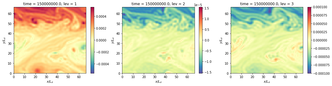
Snapshots
[7]:
PV = ds.q + ds.Qy * ds.y
PV['x'] = ds.x/ds.attrs['pyqg:rd']; PV.x.attrs = {'long_name': r'$x/L_d$'}
PV['y'] = ds.y/ds.attrs['pyqg:rd']; PV.y.attrs = {'long_name': r'$y/L_d$'}
[8]:
plt.figure(figsize=(18,4))

plt.subplot(131)
PV.sel(lev=1).plot(cmap='Spectral_r')

plt.subplot(132)
PV.sel(lev=2).plot(cmap='Spectral_r')

plt.subplot(133)
PV.sel(lev=3).plot(cmap='Spectral_r');
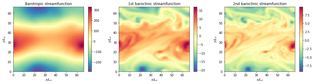
pyqg has a built-in method that computes the vertical modes. It is stored as an attribute in the Dataset.
[9]:
print(f"The first baroclinic deformation radius is {ds.attrs['pyqg:radii'][1]/1.e3} km")
print(f"The second baroclinic deformation radius is {ds.attrs['pyqg:radii'][2]/1.e3} km")
The first baroclinic deformation radius is 15.375382785987185 km
The second baroclinic deformation radius is 7.975516271996243 km
We can project the solution onto the modes
[10]:
pn = m.modal_projection(m.p)
[11]:
plt.figure(figsize=(18,4))

plt.subplot(131)
plt.pcolormesh(m.x/m.rd, m.y/m.rd, pn[0]/(U1*Ld), cmap='Spectral_r', shading='auto')
plt.xlabel(r'$x/L_d$')
plt.ylabel(r'$y/L_d$')
plt.colorbar()
plt.title('Barotropic streamfunction')

plt.subplot(132)
plt.pcolormesh(m.x/m.rd, m.y/m.rd, pn[1]/(U1*Ld), cmap='Spectral_r', shading='auto')
plt.xlabel(r'$x/L_d$')
plt.ylabel(r'$y/L_d$')
plt.colorbar()
plt.title('1st baroclinic streamfunction')

plt.subplot(133)
plt.pcolormesh(m.x/m.rd, m.y/m.rd, pn[2]/(U1*Ld), cmap='Spectral_r', shading='auto')
plt.xlabel(r'$x/L_d$')
plt.ylabel(r'$y/L_d$')
plt.colorbar()
plt.title('2nd baroclinic streamfunction');
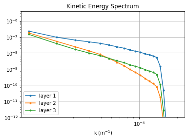
Diagnostics
[12]:
kr, kespec_1 = tools.calc_ispec(m, ds.KEspec.sel(lev=1).data.squeeze())
_ , kespec_2 = tools.calc_ispec(m, ds.KEspec.sel(lev=2).data.squeeze())
_ , kespec_3 = tools.calc_ispec(m, ds.KEspec.sel(lev=3).data.squeeze())

plt.loglog(kr, kespec_1, '.-' )
plt.loglog(kr, kespec_2, '.-' )
plt.loglog(kr, kespec_3, '.-' )

plt.legend(['layer 1','layer 2', 'layer 3'], loc='lower left')
plt.ylim([1e-12,4e-6]);
plt.xlabel(r'k (m$^{-1}$)'); plt.grid()
plt.title('Kinetic Energy Spectrum');
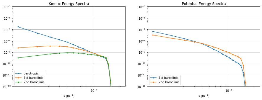
By default the modal KE and PE spectra are also calculated
[13]:
kr, modal_kespec_1 = tools.calc_ispec(m, ds.KEspec_modal.sel(lev=1).data.squeeze())
_,  modal_kespec_2 = tools.calc_ispec(m, ds.KEspec_modal.sel(lev=2).data.squeeze())
_,  modal_kespec_3 = tools.calc_ispec(m, ds.KEspec_modal.sel(lev=3).data.squeeze())

_,  modal_pespec_2 = tools.calc_ispec(m, ds.PEspec_modal.sel(lev_mid=1.5).data.squeeze())
_,  modal_pespec_3 = tools.calc_ispec(m, ds.PEspec_modal.sel(lev_mid=2.5).data.squeeze())
[14]:
plt.figure(figsize=(15,5))

plt.subplot(121)
plt.loglog(kr, modal_kespec_1, '.-')
plt.loglog(kr, modal_kespec_2, '.-')
plt.loglog(kr, modal_kespec_3, '.-')

plt.legend(['barotropic ','1st baroclinic', '2nd baroclinic'], loc='lower left')
plt.ylim([1e-12,1e-5]);
plt.xlabel(r'k (m$^{-1}$)'); plt.grid()
plt.title('Kinetic Energy Spectra');


plt.subplot(122)
plt.loglog(kr, modal_pespec_2, '.-')
plt.loglog(kr, modal_pespec_3, '.-')

plt.legend(['1st baroclinic', '2nd baroclinic'], loc='lower left')
plt.ylim([1e-12,1e-5]);
plt.xlabel(r'k (m$^{-1}$)'); plt.grid()
plt.title('Potential Energy Spectra');
[15]:
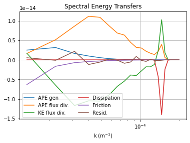
_, APEgenspec = tools.calc_ispec(m, ds.APEgenspec.data.squeeze())
_, APEflux    = tools.calc_ispec(m, ds.APEflux_div.data.squeeze())
_, KEflux     = tools.calc_ispec(m, ds.KEflux_div.data.squeeze())
_, Dissspec   = tools.calc_ispec(m, ds.Dissspec.squeeze().data)
_, KEfrictionspec = tools.calc_ispec(m, ds.KEfrictionspec.squeeze().data)

ebud = [ APEgenspec,
         APEflux,
         KEflux,
         Dissspec,
         KEfrictionspec]
ebud.append(-np.vstack(ebud).sum(axis=0))
ebud_labels = ['APE gen','APE flux div.','KE flux div.','Dissipation','Friction','Resid.']
[plt.semilogx(kr, term) for term in ebud]
plt.legend(ebud_labels, loc='lower left', ncol=2)
plt.xlabel(r'k (m$^{-1}$)'); plt.grid()
plt.title('Spectral Energy Transfers');
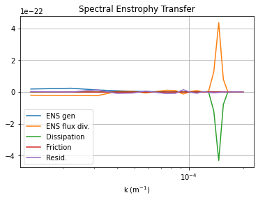
[16]:
_, ENSflux    = tools.calc_ispec(m, ds.ENSflux.data.squeeze())
_, ENSgenspec = tools.calc_ispec(m, ds.ENSgenspec.data.squeeze())
_, ENSfrictionspec = tools.calc_ispec(m, ds.ENSfrictionspec.data.squeeze())
_, ENSDissspec = tools.calc_ispec(m, ds.ENSDissspec.data.squeeze())

ebud = [ ENSgenspec,
         ENSflux,
         ENSDissspec,
         ENSfrictionspec]
ebud.append(-np.vstack(ebud).sum(axis=0))
ebud_labels = ['ENS gen','ENS flux div.','Dissipation','Friction','Resid.']
[plt.semilogx(kr, term) for term in ebud]
plt.legend(ebud_labels, loc='lower left')
plt.xlabel(r'k (m$^{-1}$)'); plt.grid()
plt.title('Spectral Enstrophy Transfer');
The dynamics here is similar to the reference experiment of Larichev & Held (1995). The APE generated through baroclinic instability is fluxed towards deformation length scales, where it is converted into KE. The KE the experiments and inverse tranfer, cascading up to the scale of the domain. The mechanical bottom drag essentially removes the large scale KE.