Built-in linear stability analysis
[11]:
import numpy as np
from numpy import pi
import matplotlib.pyplot as plt
%matplotlib inline

import pyqg
[12]:
m = pyqg.LayeredModel(nx=256, nz = 2, U = [.01, -.01], V = [0., 0.], H = [1., 1.],
                              L=2*pi,beta=1.5, rd=1./20., rek=0.05, f=1.,delta=1.)
INFO:  Logger initialized
INFO:  Kernel initialized
To perform linear stability analysis, we simply call pyqg’s built-in method stability_analysis:
[3]:
evals,evecs = m.stability_analysis()
The eigenvalues are stored in omg, and the eigenctors in evec. For plotting purposes, we use fftshift to reorder the entries
[4]:
evals = np.fft.fftshift(evals.imag,axes=(0,))

k,l = m.k*m.radii[1], np.fft.fftshift(m.l,axes=(0,))*m.radii[1]
It is also useful to analyze the fasted-growing mode:
[5]:
argmax = evals[m.Ny/2,:].argmax()
evec = np.fft.fftshift(evecs,axes=(1))[:,m.Ny/2,argmax]
kmax = k[m.Ny/2,argmax]

x = np.linspace(0,4.*pi/kmax,100)
mag, phase = np.abs(evec), np.arctan2(evec.imag,evec.real)
By default, the stability analysis above is performed without bottom friction, but the stability method also supports bottom friction:
[6]:
evals_fric, evecs_fric = m.stability_analysis(bottom_friction=True)
evals_fric = np.fft.fftshift(evals_fric.imag,axes=(0,))

argmax = evals_fric[m.Ny/2,:].argmax()
evec_fric = np.fft.fftshift(evecs_fric,axes=(1))[:,m.Ny/2,argmax]
kmax_fric = k[m.Ny/2,argmax]

mag_fric, phase_fric = np.abs(evec_fric), np.arctan2(evec_fric.imag,evec_fric.real)
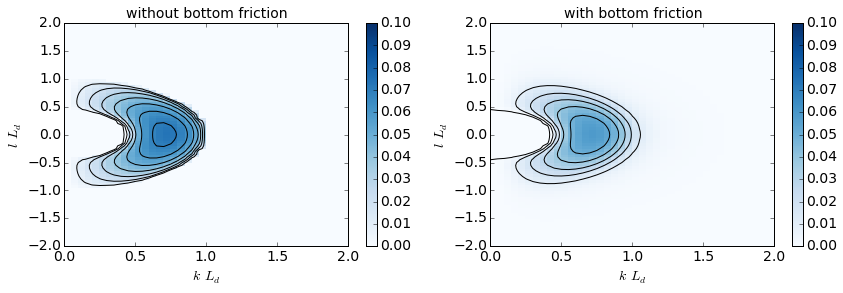
Plotting growth rates
[10]:
plt.figure(figsize=(14,4))
plt.subplot(121)
plt.contour(k,l,evals,colors='k')
plt.pcolormesh(k,l,evals,cmap='Blues')
plt.colorbar()
plt.xlim(0,2.); plt.ylim(-2.,2.)
plt.clim([0.,.1])
plt.xlabel(r'$k \, L_d$'); plt.ylabel(r'$l \, L_d$')
plt.title('without bottom friction')

plt.subplot(122)
plt.contour(k,l,evals_fric,colors='k')
plt.pcolormesh(k,l,evals_fric,cmap='Blues')
plt.colorbar()
plt.xlim(0,2.); plt.ylim(-2.,2.)
plt.clim([0.,.1])
plt.xlabel(r'$k \, L_d$'); plt.ylabel(r'$l \, L_d$')
plt.title('with bottom friction')
[10]:
<matplotlib.text.Text at 0x11539e290>
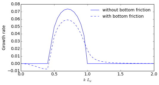
[8]:
plt.figure(figsize=(8,4))
plt.plot(k[m.Ny/2,:],evals[m.Ny/2,:],'b',label='without bottom friction')
plt.plot(k[m.Ny/2,:],evals_fric[m.Ny/2,:],'b--',label='with bottom friction')
plt.xlim(0.,2.)
plt.legend()
plt.xlabel(r'$k\,L_d$')
plt.ylabel(r'Growth rate')
[8]:
<matplotlib.text.Text at 0x10f9731d0>
Plotting the wavestructure of the most unstable modes
[9]:
plt.figure(figsize=(12,5))
plt.plot(x,mag[0]*np.cos(kmax*x + phase[0]),'b',label='Layer 1')
plt.plot(x,mag[1]*np.cos(kmax*x + phase[1]),'g',label='Layer 2')
plt.plot(x,mag_fric[0]*np.cos(kmax_fric*x + phase_fric[0]),'b--')
plt.plot(x,mag_fric[1]*np.cos(kmax_fric*x + phase_fric[1]),'g--')
plt.legend(loc=8)
plt.xlabel(r'$x/L_d$'); plt.ylabel(r'$y/L_d$')
[9]:
<matplotlib.text.Text at 0x114c6d410>
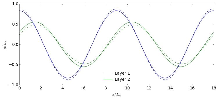
This calculation shows the classic phase-tilting of baroclinic unstable waves (e.g. Vallis 2006 ).
[ ]: