Two-Layer QG Model Example
Here is a quick overview of how to use the two-layer model. See the :py:class:pyqg.QGModel api documentation for further details.
First import numpy, matplotlib, and pyqg:
[1]:
import numpy as np
from matplotlib import pyplot as plt
%matplotlib inline

import pyqg
from pyqg import diagnostic_tools as tools
Initialize and Run the Model
Here we set up a model which will run for 10 years and start averaging after 5 years. There are lots of parameters that can be specified as keyword arguments but we are just using the defaults.
[2]:
year = 24*60*60*360.
m = pyqg.QGModel(tmax=10*year, twrite=10000, tavestart=5*year)
m.run()
INFO:  Logger initialized
INFO: Step: 10000, Time: 7.20e+07, KE: 4.14e-04, CFL: 0.090
INFO: Step: 20000, Time: 1.44e+08, KE: 4.58e-04, CFL: 0.084
INFO: Step: 30000, Time: 2.16e+08, KE: 4.35e-04, CFL: 0.109
INFO: Step: 40000, Time: 2.88e+08, KE: 4.85e-04, CFL: 0.080
Convert Model Outpt to an xarray Dataset
Model variables, coordinates, attributes, and metadata can be stored conveniently as an xarray Dataset. (Notice that this feature requires xarray to be installed on your machine. See here for installation instructions: http://xarray.pydata.org/en/stable/getting-started-guide/installing.html#instructions)
[3]:
m_ds = m.to_dataset().isel(time=-1)
m_ds
[3]:
<xarray.Dataset>
Dimensions:            (lev: 2, y: 64, x: 64, l: 64, k: 33, lev_mid: 1)
Coordinates:
    time               float64 3.11e+08
  * lev                (lev) int64 1 2
  * lev_mid            (lev_mid) float64 1.5
  * x                  (x) float64 7.812e+03 2.344e+04 ... 9.766e+05 9.922e+05
  * y                  (y) float64 7.812e+03 2.344e+04 ... 9.766e+05 9.922e+05
  * l                  (l) float64 0.0 6.283e-06 ... -1.257e-05 -6.283e-06
  * k                  (k) float64 0.0 6.283e-06 ... 0.0001948 0.0002011
Data variables: (12/32)
    q                  (lev, y, x) float64 -1.822e-06 -1.356e-06 ... -1.087e-06
    u                  (lev, y, x) float64 -0.05977 -0.04566 ... -0.001317
    v                  (lev, y, x) float64 0.04194 0.0462 ... 0.00118 0.009001
    ufull              (lev, y, x) float64 -0.03477 -0.02066 ... -0.001317
    vfull              (lev, y, x) float64 0.04194 0.0462 ... 0.00118 0.009001
    qh                 (lev, l, k) complex128 (0.002324483338567505+0j) ... (...
    ...                 ...
    ENSgenspec         (l, k) float64 0.0 -3.458e-24 ... 7.51e-52 -3.186e-61
    ENSfrictionspec    (l, k) float64 0.0 -7.479e-24 ... -2.395e-50 -7.94e-60
    APEgenspec         (l, k) float64 0.0 -7.781e-16 ... 1.69e-43 -7.168e-53
    APEflux            (l, k) float64 -0.0 -7.048e-16 ... 1.097e-28 2.951e-33
    KEflux             (l, k) float64 0.0 -4.226e-15 ... 5.188e-27 9.932e-32
    APEgen             float64 6.336e-11
Attributes: (12/23)
    pyqg:beta:       1.5e-11
    pyqg:delta:      0.25
    pyqg:del2:       0.8
    pyqg:dt:         7200.0
    pyqg:filterfac:  23.6
    pyqg:L:          1000000.0
    ...              ...
    pyqg:tc:         43200
    pyqg:tmax:       311040000.0
    pyqg:twrite:     10000
    pyqg:W:          1000000.0
    title:           pyqg: Python Quasigeostrophic Model
reference: https://pyqg.readthedocs.io/en/latest/index.html- lev: 2
- y: 64
- x: 64
- l: 64
- k: 33
- lev_mid: 1
- time()float643.11e+08
- long_name :
- model time
- units :
- s
array(3.1104e+08)
- lev(lev)int641 2
- long_name :
- vertical levels
array([1, 2])
- lev_mid(lev_mid)float641.5
- long_name :
- vertical level interface
array([1.5])
- x(x)float647.812e+03 2.344e+04 ... 9.922e+05
- long_name :
- real space grid points in the x direction
- units :
- grid point
array([ 7812.5, 23437.5, 39062.5, 54687.5, 70312.5, 85937.5, 101562.5, 117187.5, 132812.5, 148437.5, 164062.5, 179687.5, 195312.5, 210937.5, 226562.5, 242187.5, 257812.5, 273437.5, 289062.5, 304687.5, 320312.5, 335937.5, 351562.5, 367187.5, 382812.5, 398437.5, 414062.5, 429687.5, 445312.5, 460937.5, 476562.5, 492187.5, 507812.5, 523437.5, 539062.5, 554687.5, 570312.5, 585937.5, 601562.5, 617187.5, 632812.5, 648437.5, 664062.5, 679687.5, 695312.5, 710937.5, 726562.5, 742187.5, 757812.5, 773437.5, 789062.5, 804687.5, 820312.5, 835937.5, 851562.5, 867187.5, 882812.5, 898437.5, 914062.5, 929687.5, 945312.5, 960937.5, 976562.5, 992187.5]) - y(y)float647.812e+03 2.344e+04 ... 9.922e+05
- long_name :
- real space grid points in the y direction
- units :
- grid point
array([ 7812.5, 23437.5, 39062.5, 54687.5, 70312.5, 85937.5, 101562.5, 117187.5, 132812.5, 148437.5, 164062.5, 179687.5, 195312.5, 210937.5, 226562.5, 242187.5, 257812.5, 273437.5, 289062.5, 304687.5, 320312.5, 335937.5, 351562.5, 367187.5, 382812.5, 398437.5, 414062.5, 429687.5, 445312.5, 460937.5, 476562.5, 492187.5, 507812.5, 523437.5, 539062.5, 554687.5, 570312.5, 585937.5, 601562.5, 617187.5, 632812.5, 648437.5, 664062.5, 679687.5, 695312.5, 710937.5, 726562.5, 742187.5, 757812.5, 773437.5, 789062.5, 804687.5, 820312.5, 835937.5, 851562.5, 867187.5, 882812.5, 898437.5, 914062.5, 929687.5, 945312.5, 960937.5, 976562.5, 992187.5]) - l(l)float640.0 6.283e-06 ... -6.283e-06
- long_name :
- spectal space grid points in the l direction
- units :
- meridional wavenumber
array([ 0.000000e+00, 6.283185e-06, 1.256637e-05, 1.884956e-05, 2.513274e-05, 3.141593e-05, 3.769911e-05, 4.398230e-05, 5.026548e-05, 5.654867e-05, 6.283185e-05, 6.911504e-05, 7.539822e-05, 8.168141e-05, 8.796459e-05, 9.424778e-05, 1.005310e-04, 1.068142e-04, 1.130973e-04, 1.193805e-04, 1.256637e-04, 1.319469e-04, 1.382301e-04, 1.445133e-04, 1.507964e-04, 1.570796e-04, 1.633628e-04, 1.696460e-04, 1.759292e-04, 1.822124e-04, 1.884956e-04, 1.947787e-04, -2.010619e-04, -1.947787e-04, -1.884956e-04, -1.822124e-04, -1.759292e-04, -1.696460e-04, -1.633628e-04, -1.570796e-04, -1.507964e-04, -1.445133e-04, -1.382301e-04, -1.319469e-04, -1.256637e-04, -1.193805e-04, -1.130973e-04, -1.068142e-04, -1.005310e-04, -9.424778e-05, -8.796459e-05, -8.168141e-05, -7.539822e-05, -6.911504e-05, -6.283185e-05, -5.654867e-05, -5.026548e-05, -4.398230e-05, -3.769911e-05, -3.141593e-05, -2.513274e-05, -1.884956e-05, -1.256637e-05, -6.283185e-06]) - k(k)float640.0 6.283e-06 ... 0.0002011
- long_name :
- spectal space grid points in the k direction
- units :
- zonal wavenumber
array([0.000000e+00, 6.283185e-06, 1.256637e-05, 1.884956e-05, 2.513274e-05,
       3.141593e-05, 3.769911e-05, 4.398230e-05, 5.026548e-05, 5.654867e-05,
       6.283185e-05, 6.911504e-05, 7.539822e-05, 8.168141e-05, 8.796459e-05,
       9.424778e-05, 1.005310e-04, 1.068142e-04, 1.130973e-04, 1.193805e-04,
       1.256637e-04, 1.319469e-04, 1.382301e-04, 1.445133e-04, 1.507964e-04,
       1.570796e-04, 1.633628e-04, 1.696460e-04, 1.759292e-04, 1.822124e-04,
       1.884956e-04, 1.947787e-04, 2.010619e-04])
- q(lev, y, x)float64-1.822e-06 ... -1.087e-06
- units :
- s^-1
- long_name :
- potential vorticity in real space
array([[[-1.82155607e-06, -1.35614850e-06, -2.73898371e-06, ..., -6.85958828e-06, -3.88652325e-06, -7.07170613e-07], [-2.24241759e-06, -6.30783618e-06, -9.64180522e-06, ..., 8.28700407e-07, -3.62581851e-06, -2.18831772e-06], [-3.21053920e-06, -1.23838527e-05, -1.70457033e-05, ..., 5.90566987e-06, -4.37522563e-06, -3.90119075e-06], ..., [ 1.74383701e-05, 4.74421973e-06, -3.97541428e-06, ..., 1.39955471e-05, 2.88647068e-05, 2.92223526e-05], [ 1.63871061e-05, 4.98120523e-06, -3.30331793e-06, ..., 7.80011160e-06, 2.43203864e-05, 2.74599319e-05], [ 4.29350266e-06, -1.76233514e-07, -4.52788793e-06, ..., -4.09975671e-06, 6.90339664e-06, 1.07226221e-05]], [[-3.33208786e-08, 3.96628369e-07, 7.16963768e-07, ..., 5.78802928e-07, 3.48351068e-07, -1.59284286e-07], [ 8.82458643e-07, 1.40627384e-06, 1.61550730e-06, ..., 6.19656450e-07, 8.79536706e-07, 6.72872557e-07], [ 1.72684105e-06, 2.07050296e-06, 1.79271303e-06, ..., 3.44060815e-07, 1.19072781e-06, 1.45201173e-06], ..., [-1.96770868e-06, -6.02974769e-07, -1.93654523e-07, ..., -1.71781896e-06, -2.97724536e-06, -3.21060907e-06], [-1.53072205e-06, -4.76886961e-07, -1.02493765e-07, ..., -9.52231342e-07, -1.92618338e-06, -2.37473090e-06], [-6.82081661e-07, -1.07404161e-07, 1.63025070e-07, ..., -1.65139673e-07, -6.49227654e-07, -1.08681543e-06]]]) - u(lev, y, x)float64-0.05977 -0.04566 ... -0.001317
- units :
- m s^-1
- long_name :
- zonal velocity anomaly
array([[[-0.05977365, -0.04566044, -0.0300013 , ..., 0.00313956, -0.05354602, -0.07361268], [-0.03410872, -0.04832014, -0.0436795 , ..., 0.03619708, -0.00852563, -0.0302402 ], [-0.01284595, -0.0007373 , 0.01982649, ..., 0.00808109, -0.01780913, -0.02519738], ..., [ 0.03291048, 0.01935363, 0.00108856, ..., -0.01936507, 0.01178554, 0.03422701], [-0.06464542, -0.03662093, -0.02514983, ..., -0.07523594, -0.09564462, -0.08762571], [-0.09744367, -0.05272586, -0.02502093, ..., -0.06773183, -0.12211898, -0.13019829]], [[ 0.00018518, 0.00178978, 0.00374121, ..., 0.00738511, 0.0028788 , 0.00019862], [ 0.0026525 , 0.00251875, 0.00221745, ..., 0.00521121, 0.00308351, 0.00242911], [-0.00196729, -0.00190097, -0.00146095, ..., 0.00088748, -0.00132439, -0.00201614], ..., [ 0.00593403, 0.00365724, 0.0017545 , ..., 0.01161436, 0.0113088 , 0.00879691], [ 0.00172549, 0.00071104, 0.00080111, ..., 0.00678718, 0.00541306, 0.00367907], [-0.00198774, -0.00057552, 0.00172088, ..., 0.00614775, 0.00158964, -0.00131667]]]) - v(lev, y, x)float640.04194 0.0462 ... 0.00118 0.009001
- units :
- m s^-1
- long_name :
- meridional velocity anomaly
array([[[ 0.04193728, 0.04619567, 0.04606487, ..., 0.00914963, -0.01375966, 0.01612357], [ 0.04114261, 0.04963187, 0.02388613, ..., 0.05653599, 0.029679 , 0.01889034], [ 0.04238221, 0.05254364, -0.00317824, ..., 0.08718173, 0.06116157, 0.0193422 ], ..., [ 0.12361364, 0.11601851, 0.05419519, ..., -0.11855288, -0.06021382, 0.05868665], [ 0.11444405, 0.11155098, 0.06699201, ..., -0.11226167, -0.07512554, 0.04453635], [ 0.07533527, 0.07553595, 0.06256184, ..., -0.05571866, -0.05462336, 0.02682797]], [[ 0.01243645, 0.01307927, 0.01055738, ..., -0.00193764, 0.00550631, 0.01063706], [ 0.011838 , 0.01226643, 0.0098713 , ..., 0.00129449, 0.00826311, 0.01119273], [ 0.01187803, 0.01273346, 0.00989068, ..., 0.00367322, 0.00943853, 0.01105163], ..., [ 0.01046388, 0.01504644, 0.01335022, ..., -0.01056941, -0.0026157 , 0.00459572], [ 0.01279311, 0.01647135, 0.01391478, ..., -0.01038098, -0.0014363 , 0.00714923], [ 0.01334085, 0.01548231, 0.01263995, ..., -0.00688463, 0.00118041, 0.00900085]]]) - ufull(lev, y, x)float64-0.03477 -0.02066 ... -0.001317
- units :
- m s^-1
- long_name :
- zonal full velocities in real space
array([[[-3.47736519e-02, -2.06604356e-02, -5.00130117e-03, ..., 2.81395648e-02, -2.85460236e-02, -4.86126789e-02], [-9.10872099e-03, -2.33201399e-02, -1.86794994e-02, ..., 6.11970801e-02, 1.64743670e-02, -5.24020014e-03], [ 1.21540536e-02, 2.42627049e-02, 4.48264878e-02, ..., 3.30810948e-02, 7.19086952e-03, -1.97384631e-04], ..., [ 5.79104757e-02, 4.43536257e-02, 2.60885571e-02, ..., 5.63492850e-03, 3.67855361e-02, 5.92270089e-02], [-3.96454245e-02, -1.16209314e-02, -1.49831987e-04, ..., -5.02359400e-02, -7.06446179e-02, -6.26257108e-02], [-7.24436689e-02, -2.77258637e-02, -2.09251419e-05, ..., -4.27318328e-02, -9.71189759e-02, -1.05198294e-01]], [[ 1.85178683e-04, 1.78978348e-03, 3.74121000e-03, ..., 7.38511443e-03, 2.87879559e-03, 1.98623349e-04], [ 2.65249705e-03, 2.51874738e-03, 2.21744836e-03, ..., 5.21121011e-03, 3.08350991e-03, 2.42910507e-03], [-1.96729014e-03, -1.90096873e-03, -1.46095285e-03, ..., 8.87477936e-04, -1.32439200e-03, -2.01613867e-03], ..., [ 5.93402695e-03, 3.65723784e-03, 1.75449644e-03, ..., 1.16143622e-02, 1.13088014e-02, 8.79691414e-03], [ 1.72549331e-03, 7.11035015e-04, 8.01114513e-04, ..., 6.78717670e-03, 5.41306198e-03, 3.67906691e-03], [-1.98774402e-03, -5.75520802e-04, 1.72088364e-03, ..., 6.14775491e-03, 1.58963584e-03, -1.31666776e-03]]]) - vfull(lev, y, x)float640.04194 0.0462 ... 0.00118 0.009001
- units :
- m s^-1
- long_name :
- meridional full velocities in real space
array([[[ 0.04193728, 0.04619567, 0.04606487, ..., 0.00914963, -0.01375966, 0.01612357], [ 0.04114261, 0.04963187, 0.02388613, ..., 0.05653599, 0.029679 , 0.01889034], [ 0.04238221, 0.05254364, -0.00317824, ..., 0.08718173, 0.06116157, 0.0193422 ], ..., [ 0.12361364, 0.11601851, 0.05419519, ..., -0.11855288, -0.06021382, 0.05868665], [ 0.11444405, 0.11155098, 0.06699201, ..., -0.11226167, -0.07512554, 0.04453635], [ 0.07533527, 0.07553595, 0.06256184, ..., -0.05571866, -0.05462336, 0.02682797]], [[ 0.01243645, 0.01307927, 0.01055738, ..., -0.00193764, 0.00550631, 0.01063706], [ 0.011838 , 0.01226643, 0.0098713 , ..., 0.00129449, 0.00826311, 0.01119273], [ 0.01187803, 0.01273346, 0.00989068, ..., 0.00367322, 0.00943853, 0.01105163], ..., [ 0.01046388, 0.01504644, 0.01335022, ..., -0.01056941, -0.0026157 , 0.00459572], [ 0.01279311, 0.01647135, 0.01391478, ..., -0.01038098, -0.0014363 , 0.00714923], [ 0.01334085, 0.01548231, 0.01263995, ..., -0.00688463, 0.00118041, 0.00900085]]]) - qh(lev, l, k)complex128(0.002324483338567505+0j) ... (1...
- units :
- s^-1
- long_name :
- potential vorticity in spectral space
array([[[ 2.32448334e-03+0.00000000e+00j, -2.01080652e-04-4.39246062e-04j, 1.53507095e-06-4.20067097e-04j, ..., -1.88224155e-13-2.96311988e-14j, 4.81504240e-19+7.99759315e-17j, -2.99366079e-39+8.39283127e-22j], [-2.92698757e-05+6.03290076e-04j, 3.54793590e-04-2.18449154e-04j, 2.52214672e-04-6.59930446e-04j, ..., 1.53815216e-13+1.37469143e-13j, -4.35998761e-18+5.83709453e-17j, 2.99540575e-22-2.85357222e-21j], [ 1.61731739e-04-4.20079560e-04j, -3.52313525e-04-1.40295854e-03j, -1.63231762e-04+1.19696946e-04j, ..., 1.57661809e-13+1.02150932e-14j, -8.23400906e-18+1.95994567e-17j, -1.00792612e-22+3.41673650e-23j], ..., [-5.07721866e-04+7.06202015e-04j, ... 5.61805921e-25-3.75140125e-24j], ..., [ 1.25318320e-04-1.13117572e-04j, -4.13985393e-05-2.14296869e-04j, -6.92306404e-05-3.21572049e-04j, ..., -3.21334959e-16+2.00064599e-15j, -2.82240831e-19+1.75246158e-19j, -4.59744663e-26+2.41891379e-24j], [-3.94528728e-05-6.97557545e-05j, -8.26298616e-05-1.49572101e-04j, -1.51381577e-06+1.02187434e-04j, ..., -2.25358031e-15+4.69900069e-16j, -6.06306978e-19-5.99679682e-20j, 2.29114870e-24-1.20154019e-23j], [ 1.61796735e-05+1.51818655e-04j, -1.80918831e-04+1.26499881e-04j, 3.47977208e-05+1.33735499e-05j, ..., -3.73818518e-15-2.34062717e-15j, 4.19934011e-19+1.72112874e-19j, 1.10348835e-23-1.56631921e-23j]]]) - uh(lev, l, k)complex128(-39.060809062416254+0j) ... (-3...
- units :
- m s^-1
- long_name :
- zonal velocity anomaly in spectral space
array([[[-3.90608091e+01+0.00000000e+00j, -2.06762906e+01+1.73508184e+00j, 4.33688640e-01-2.14771838e-01j, ..., 1.20237434e-10+1.22581925e-10j, 2.28539517e-15+2.73638235e-15j, -6.45781388e-20+8.86671913e-21j], [-5.36504824e+01+0.00000000e+00j, 4.42635776e+01+1.23506486e+01j, 1.59365016e+00-3.68557154e+01j, ..., 1.38348463e-10+5.36994501e-11j, -3.52695867e-15+9.06979097e-15j, -4.58348613e-20-2.80942762e-20j], [-2.43280935e+01+0.00000000e+00j, 6.05477733e+01+2.63166040e+01j, 1.99101198e+01-5.03374383e+01j, ..., 1.39460656e-10-1.27539634e-11j, -8.67019583e-15+1.28067803e-14j, -6.33284742e-21-3.18590336e-20j], ..., [ 2.16311873e+01+0.00000000e+00j, ... -1.18888656e-21-5.59150242e-21j], ..., [ 1.17224678e+01+0.00000000e+00j, 2.64593929e+00+1.04069626e+00j, 1.11685906e+00+1.07864755e+01j, ..., -5.52563727e-13+8.68411985e-12j, 3.11153601e-16-4.04157995e-17j, -3.37784983e-21-2.88531117e-21j], [ 1.05227718e+01+0.00000000e+00j, 1.75781290e+00+3.76923449e+00j, -2.50040215e+00+1.37087074e+01j, ..., 8.35615361e-13+8.02149223e-12j, 2.73193112e-16+8.86981249e-17j, -3.92037924e-21-4.41225480e-21j], [ 7.45468949e+00+0.00000000e+00j, 2.81806951e+00+2.53775347e+00j, -6.03130177e+00+1.19614280e+01j, ..., 2.23652133e-12+6.73751338e-12j, 2.17448314e-16+2.39055914e-16j, -3.99705064e-21-5.87229612e-21j]]]) - vh(lev, l, k)complex1280j ... (-6.292253685240078e-19+2...
- units :
- m s^-1
- long_name :
- meridional velocity anomaly in spectral space
array([[[ 0.00000000e+00+0.00000000e+00j, -6.66629764e+00+5.79419093e+00j, 1.64939478e+01+1.14129578e+01j, ..., 3.43813642e-09+2.67534196e-10j, 8.36021263e-13-2.69732499e-13j, -1.57814876e-17+1.90007327e-18j], [ 0.00000000e+00+0.00000000e+00j, -6.10275592e+00+4.51854646e+00j, 1.24385903e+01+1.09167008e+01j, ..., 3.69830502e-09-1.17137135e-10j, 8.54494298e-13-2.67735299e-13j, -1.58190468e-17+2.07918491e-18j], [ 0.00000000e+00+0.00000000e+00j, -4.17163618e+00-1.20822021e+00j, 3.44705889e+00+9.42864910e+00j, ..., 3.75688547e-09-5.30597908e-10j, 8.88579094e-13-2.48947942e-13j, -1.59230525e-17+2.16621624e-18j], ..., [ 0.00000000e+00+0.00000000e+00j, ... -6.90713823e-19+5.15410688e-20j], ..., [ 0.00000000e+00+0.00000000e+00j, -1.50221707e+00-6.33378379e-02j, -6.88126379e-01-3.38280925e+00j, ..., 3.05134435e-11+4.92047404e-11j, 2.19881105e-14-3.81314386e-15j, -6.01572655e-19-4.29386170e-22j], [ 0.00000000e+00+0.00000000e+00j, -1.23586877e+00-2.74358125e-01j, 1.76314072e+00-3.29207121e+00j, ..., 5.52800561e-11+4.88205516e-11j, 2.20529085e-14-4.70788341e-15j, -6.12989209e-19+1.11449488e-20j], [ 0.00000000e+00+0.00000000e+00j, -8.99957764e-01-4.75333696e-01j, 4.38081381e+00-2.41531668e+00j, ..., 7.71509683e-11+4.42692766e-11j, 2.25497652e-14-5.45793111e-15j, -6.29225369e-19+2.37134782e-20j]]]) - ph(lev, l, k)complex1280j ... (-9.114747217910704e-17+1...
- units :
- m^2 s^-1
- long_name :
- streamfunction in spectral space
array([[[ 0.00000000e+00+0.00000000e+00j, 8.39975810e+04+1.00692609e+05j, -2.25032933e+04+7.30426384e+03j, ..., 4.78122204e-06+7.81118780e-07j, -2.69136901e-11-1.92528717e-09j, 6.83339794e-32-1.91152085e-14j], [-1.71543723e+05-1.14820851e+05j, -1.15392094e+05+9.46613399e+04j, -1.49294292e+05+2.04864604e+05j, ..., -3.81431846e-06-3.67850126e-06j, 1.56187433e-10-1.35359732e-09j, -7.06969307e-15+6.48995002e-14j], [-3.95191801e+04+2.63444806e+05j, -2.28589604e+04+4.77298129e+05j, 2.05192125e+04-1.66583547e+04j, ..., -4.03558234e-06-3.65470935e-07j, 2.07110353e-10-4.32175766e-10j, 1.07638255e-15-1.10020492e-15j], ..., [ 1.09370696e+05-2.79500412e+05j, ... 1.09978828e-17+6.16270605e-17j], ..., [-2.25961145e+04-1.08660256e+05j, -6.11750802e+02-1.54582008e+05j, -5.41566103e+04-8.65925364e+04j, ..., 8.01713256e-08-6.67041565e-08j, -1.56242319e-12+4.46067683e-12j, -9.12967879e-17-6.35761311e-17j], [ 3.90714535e+03-1.57168781e+05j, 7.63897180e+04+3.48593962e+04j, 1.47666318e+05+8.44959665e+03j, ..., 5.95741166e-08-1.54408134e-07j, 1.64482508e-11-4.77368441e-12j, 1.86708714e-16+1.38160987e-16j], [-1.81675230e+05-5.36556727e+04j, -9.11610787e+04+2.74125502e+04j, -1.36354890e+05-2.71384385e+02j, ..., 8.79005445e-08-5.65019610e-08j, -2.77429959e-11-4.36824600e-11j, -9.11474722e-17+1.52245960e-15j]]]) - dqhdt(lev, l, k)complex128(-0-0j) ... (1.7617742214702241e...
- units :
- s^-2
- long_name :
- previous partial derivative of potential vorticity wrt. time in spectral space
array([[[-0.00000000e+00-0.00000000e+00j, -3.86764655e-11-7.68358643e-12j, -1.40536833e-10+1.50126986e-10j, ..., -1.72320643e-10-2.75723086e-11j, 2.24516032e-12+2.24370494e-10j, -3.99280395e-28+1.11941857e-10j], [-2.75534890e-12-3.76298518e-11j, -3.73486844e-11-4.22377984e-11j, 3.37755096e-11+8.10649340e-11j, ..., 1.56137258e-10+1.44752900e-10j, -1.77896313e-11+1.86998273e-10j, 4.93537691e-11-4.60848056e-10j], [ 1.50982658e-10-8.47125976e-11j, 1.54275188e-10+1.65761530e-10j, -2.80712916e-11-7.36408243e-11j, ..., 2.29786125e-10+1.78063142e-11j, -4.34630303e-11+9.68319595e-11j, -2.14306548e-11+1.20467462e-11j], ..., [ 4.88094845e-11-7.46402415e-11j, ... 1.53944643e-13-1.05406334e-12j], ..., [-1.91300325e-12+1.84361759e-11j, -4.69792647e-11-5.49828626e-12j, 5.84761435e-12-2.43811081e-11j, ..., -8.46643650e-13+5.23244563e-12j, -3.13536764e-12+1.94549683e-12j, -4.08659085e-14+1.85082940e-12j], [-3.25807491e-11-1.49158466e-11j, -1.60679566e-11+3.31564556e-11j, 1.51118326e-11+5.38873773e-12j, ..., -3.27891862e-12+6.86330006e-13j, -3.10204959e-12-3.04848569e-13j, 6.71792676e-13-3.45260401e-12j], [ 2.42821648e-13-7.85083198e-12j, -2.31744952e-11-1.49179172e-11j, -2.90741823e-11-1.99008647e-11j, ..., -3.85216251e-12-2.43477494e-12j, 1.36240518e-12+5.80086651e-13j, 1.76177422e-12-2.50264620e-12j]]]) - Ubg(lev)float640.025 0.0
- units :
- m s^-1
- long_name :
- background zonal velocity
array([0.025, 0. ])
- Qy(lev)float641.039e-10 -7.222e-12
- units :
- m^-1 s^-1
- long_name :
- background potential vorticity gradient
array([ 1.03888889e-10, -7.22222222e-12])
- dqdt(lev, y, x)float64-7.465e-12 ... -8.823e-13
- units :
- s^-2
- long_name :
- previous partial derivative of potential vorticity wrt. time in real space
array([[[-7.46480121e-12, -7.05301364e-12, -2.50852789e-12, ..., 8.10469953e-12, -3.17683647e-12, 2.73974577e-12], [-2.76997848e-12, 2.17936883e-11, 9.59576924e-12, ..., -1.13352671e-11, 1.63170042e-12, 4.22105886e-12], [-4.82795936e-13, 1.12061876e-11, -5.79556648e-12, ..., 9.42784264e-12, 7.15595642e-12, -4.68795757e-12], ..., [-1.06603635e-11, -5.81864791e-12, -7.50220858e-12, ..., -1.27884657e-11, 1.43449582e-11, -5.26804162e-12], [ 2.11718134e-11, 4.52763323e-12, 1.22028997e-12, ..., -1.43204608e-11, -7.71830287e-12, -6.75550187e-13], [ 1.81453295e-11, 1.18766938e-11, -1.23646569e-11, ..., -1.06645633e-11, 1.67536304e-11, 8.48204329e-12]], [[-3.27685950e-13, -4.08228921e-13, -3.16244516e-13, ..., -3.05938150e-13, -2.98492814e-13, -4.37900110e-13], [-8.92131814e-13, -9.65029971e-13, -3.94851240e-13, ..., -6.34837154e-13, -3.82828419e-13, -6.20347624e-13], [-4.29263534e-13, -2.22594932e-14, 4.68287952e-13, ..., -4.44701468e-13, -3.74553750e-13, -5.39096719e-13], ..., [-7.91955099e-13, -2.01448024e-13, 3.18076661e-13, ..., 1.10272854e-12, 3.83546108e-13, -6.88516473e-13], [-1.08710988e-12, -3.62382375e-13, 1.50900153e-13, ..., 3.73534447e-13, -1.83579735e-13, -1.06252388e-12], [-6.32057816e-13, -2.68329613e-13, 6.63375808e-14, ..., 2.36160060e-13, -3.85837772e-13, -8.82316262e-13]]]) - p(lev, y, x)float64-247.4 450.7 ... -705.3 -621.2
- units :
- m^2 s^-1
- long_name :
- streamfunction in real space
array([[[-2.47381527e+02, 4.50686452e+02, 1.18462755e+03, ..., -6.13686454e+02, -7.16347205e+02, -7.40135279e+02], [ 4.55907305e+02, 1.21151360e+03, 1.81812317e+03, ..., -1.01901104e+03, -3.20375578e+02, 4.26449504e+00], [ 8.34947519e+02, 1.66696358e+03, 2.10119915e+03, ..., -1.40717066e+03, -1.47115787e+02, 4.16884061e+02], ..., [-3.15532332e+03, -1.20408874e+03, 1.85240148e+02, ..., -3.14075295e+03, -4.68167353e+03, -4.68662633e+03], [-2.90503063e+03, -1.07218303e+03, 3.69820356e+02, ..., -2.37614482e+03, -4.00664292e+03, -4.26189567e+03], [-1.50142416e+03, -2.95536991e+02, 8.05719400e+02, ..., -1.13731174e+03, -2.13932315e+03, -2.38926491e+03]], [[-4.22566434e+02, -2.21382990e+02, -3.06375994e+01, ..., -7.64257789e+02, -7.36823014e+02, -6.05208458e+02], [-4.51020676e+02, -2.61408427e+02, -8.28712847e+01, ..., -8.67400820e+02, -7.88825602e+02, -6.31425892e+02], [-4.65884218e+02, -2.71415905e+02, -8.80387724e+01, ..., -9.15972952e+02, -8.07781808e+02, -6.43859705e+02], ..., [-3.87079982e+02, -1.83538037e+02, 4.94190574e+01, ..., -4.18870074e+02, -5.23407333e+02, -5.05290616e+02], [-4.51463465e+02, -2.18551413e+02, 2.99736632e+01, ..., -5.61994310e+02, -6.58579830e+02, -6.09695633e+02], [-4.43276966e+02, -2.14427844e+02, 1.40496066e+01, ..., -6.56006738e+02, -7.05254610e+02, -6.21180587e+02]]]) - Ensspec(lev, l, k)float643.221e-13 3.714e-14 ... 2.195e-53
- long_name :
- enstrophy spectrum
- units :
- s^-2
array([[[3.22057175e-13, 3.71403542e-14, 2.16930481e-14, ..., 5.71871690e-33, 4.36189560e-40, 1.46392698e-49], [1.79426521e-14, 2.93879362e-14, 2.75107173e-14, ..., 4.44877708e-33, 3.10819945e-40, 1.47960701e-49], [3.87727581e-14, 2.83845192e-14, 3.34693556e-14, ..., 2.55274957e-33, 2.03372844e-40, 7.35682386e-50], ..., [9.62502459e-14, 8.53490518e-14, 1.06223689e-13, ..., 1.04755599e-33, 6.30340981e-41, 1.56764288e-50], [3.87727581e-14, 3.65703075e-14, 3.49163776e-14, ..., 2.98042516e-33, 1.97337790e-40, 7.79488065e-50], [1.79426521e-14, 2.10737124e-14, 1.77783346e-14, ..., 4.07652941e-33, 3.45020117e-40, 1.46220667e-49]], [[0.00000000e+00, 2.31037571e-15, 1.24686096e-15, ..., 9.69650234e-37, 7.77313383e-44, 2.75778178e-53], [1.08733063e-15, 1.80265152e-15, 1.47732661e-15, ..., 8.31423477e-37, 5.82516248e-44, 2.33262027e-53], [2.07080859e-15, 1.45642460e-15, 1.56012498e-15, ..., 4.10478878e-37, 2.87790905e-44, 8.22526289e-54], ..., [4.21663754e-15, 3.11157315e-15, 4.00824057e-15, ..., 1.50166582e-37, 7.04172900e-45, 1.52247195e-54], [2.07080859e-15, 1.92848905e-15, 1.48922901e-15, ..., 4.05469347e-37, 2.90864034e-44, 8.71432147e-54], [1.08733063e-15, 1.26457034e-15, 9.66235126e-16, ..., 9.34703284e-37, 6.26169709e-44, 2.19453275e-53]]]) - KEspec(lev, l, k)float640.0 8.622e-08 ... 1.725e-45
- long_name :
- kinetic energy spectrum
- units :
- m^2 s^-2
array([[[0.00000000e+00, 8.62165368e-08, 3.11562419e-07, ..., 1.33563127e-25, 9.64652925e-33, 3.06975796e-42], [1.17490940e-07, 1.82906861e-07, 5.69717366e-07, ..., 1.03818586e-25, 6.86955544e-33, 3.09942269e-42], [7.91357529e-07, 7.41483970e-07, 1.15445554e-06, ..., 5.93960597e-26, 4.48171261e-33, 1.53749040e-42], ..., [3.22695389e-06, 3.79626070e-06, 4.63974930e-06, ..., 2.42662005e-26, 1.38315605e-33, 3.26244688e-43], [7.91357529e-07, 7.96539073e-07, 1.33668827e-06, ..., 6.93511898e-26, 4.34917658e-33, 1.62897212e-42], [1.17490940e-07, 1.69667966e-07, 4.12790311e-07, ..., 9.51322177e-26, 7.62383975e-33, 3.06316983e-42]], [[0.00000000e+00, 8.01302815e-09, 5.90111062e-08, ..., 9.74026612e-29, 6.33055858e-36, 1.98539033e-45], [5.24011894e-08, 4.40332956e-08, 1.09956400e-07, ..., 8.05275074e-29, 5.00104097e-36, 1.71949441e-45], [1.91841201e-07, 1.95695441e-07, 2.22918844e-07, ..., 4.07156653e-29, 2.63519601e-36, 8.25966581e-46], ..., [2.83931580e-07, 4.90116555e-07, 3.55646425e-07, ..., 1.68504259e-29, 7.78720614e-37, 1.59739577e-46], [1.91841201e-07, 1.53728699e-07, 2.45466546e-07, ..., 4.66898159e-29, 2.70850041e-36, 8.57292827e-46], [5.24011894e-08, 4.44092019e-08, 1.18183997e-07, ..., 7.85764035e-29, 5.07577067e-36, 1.72538781e-45]]]) - EKEdiss()float645.262e-11
- long_name :
- total energy dissipation by bottom drag
- units :
- m^2 s^-3
array(5.2620925e-11)
- KEfrictionspec(l, k)float64-0.0 -3.71e-15 ... -7.988e-52
- long_name :
- total energy dissipation spectrum by bottom drag
- units :
- m^2 s^-3
array([[-0.00000000e+00, -3.70971151e-15, -2.73197817e-14, ..., -4.50935360e-35, -2.93079540e-42, -9.19156307e-52], [-2.42596547e-14, -2.03856545e-14, -5.09054149e-14, ..., -3.72810148e-35, -2.31528193e-42, -7.96057134e-52], [-8.88148024e-14, -9.05991611e-14, -1.03202508e-13, ..., -1.88497244e-35, -1.21999034e-42, -3.82389489e-52], ..., [-1.31448964e-13, -2.26904360e-13, -1.64650069e-13, ..., -7.80107316e-36, -3.60516495e-43, -7.39530344e-53], [-8.88148024e-14, -7.11702383e-14, -1.13641192e-13, ..., -2.16155172e-35, -1.25392735e-42, -3.96892287e-52], [-2.42596547e-14, -2.05596841e-14, -5.47144633e-14, ..., -3.63777318e-35, -2.34987879e-42, -7.98785540e-52]]) - EKE(lev)float640.002105 5.683e-05
- long_name :
- mean eddy kinetic energy
- units :
- m^2 s^-2
array([2.10465295e-03, 5.68309627e-05])
- Dissspec(l, k)float64-0.0 -0.0 ... -5.44e-27 -1.075e-31
- long_name :
- Spectral contribution of filter dissipation to total energy
- units :
- m^2 s^-3
array([[-0.00000000e+00, -0.00000000e+00, -0.00000000e+00, ..., -2.69775429e-23, -5.92222478e-27, -8.88727114e-32], [-0.00000000e+00, -0.00000000e+00, -0.00000000e+00, ..., -2.35027121e-23, -4.90135766e-27, -1.08815499e-31], [-0.00000000e+00, -0.00000000e+00, -0.00000000e+00, ..., -1.89904693e-23, -5.03809118e-27, -9.66362169e-32], ..., [-0.00000000e+00, -0.00000000e+00, -0.00000000e+00, ..., -1.39497309e-23, -3.36051678e-27, -5.49266578e-32], [-0.00000000e+00, -0.00000000e+00, -0.00000000e+00, ..., -2.21700749e-23, -4.88937886e-27, -1.02374670e-31], [-0.00000000e+00, -0.00000000e+00, -0.00000000e+00, ..., -2.15408317e-23, -5.43969706e-27, -1.07527907e-31]]) - ENSDissspec(l, k)float640.0 0.0 ... -2.255e-34 -4.726e-39
- long_name :
- Spectral contribution of filter dissipation to barotropic enstrophy
- units :
- s^-3
array([[ 0.00000000e+00, 0.00000000e+00, 0.00000000e+00, ..., -1.05229705e-30, -2.45310248e-34, -3.90219837e-39], [ 0.00000000e+00, 0.00000000e+00, 0.00000000e+00, ..., -9.17586872e-31, -2.03169873e-34, -4.78319490e-39], [ 0.00000000e+00, 0.00000000e+00, 0.00000000e+00, ..., -7.43837659e-31, -2.09504579e-34, -4.25875740e-39], ..., [ 0.00000000e+00, 0.00000000e+00, 0.00000000e+00, ..., -5.49088088e-31, -1.40402683e-34, -2.43173373e-39], [ 0.00000000e+00, 0.00000000e+00, 0.00000000e+00, ..., -8.68333159e-31, -2.03298790e-34, -4.51183698e-39], [ 0.00000000e+00, 0.00000000e+00, 0.00000000e+00, ..., -8.40976585e-31, -2.25532253e-34, -4.72630221e-39]]) - paramspec(l, k)float64-0.0 -0.0 -0.0 ... -0.0 -0.0 -0.0
- long_name :
- Spectral contribution of subgrid parameterization (if present)
- units :
- m^2 s^-3
array([[-0., -0., -0., ..., -0., -0., -0.], [-0., -0., -0., ..., -0., -0., -0.], [-0., -0., -0., ..., -0., -0., -0.], ..., [-0., -0., -0., ..., -0., -0., -0.], [-0., -0., -0., ..., -0., -0., -0.], [-0., -0., -0., ..., -0., -0., -0.]]) - entspec(l, k)float641.288e-14 2.147e-19 ... 5.792e-51
- long_name :
- barotropic enstrophy spectrum
- units :
- m s^-2
array([[1.28822870e-14, 2.14741640e-19, 1.10258362e-17, ..., 2.27206968e-34, 1.72932417e-41, 5.84298924e-51], [2.23721116e-18, 3.44058548e-18, 2.78185191e-17, ..., 1.77556061e-34, 1.24516247e-41, 5.84432213e-51], [3.81940910e-17, 4.78894668e-17, 9.47022603e-17, ..., 1.00956523e-34, 8.02829297e-42, 2.92275872e-51], ..., [1.87069991e-16, 3.26534785e-16, 3.64131721e-16, ..., 4.16435241e-35, 2.49288871e-42, 6.19689067e-52], [3.81940910e-17, 3.97777065e-17, 1.10957315e-16, ..., 1.18120900e-34, 7.82723106e-42, 3.09080594e-51], [2.23721116e-18, 3.89320480e-18, 2.71806541e-17, ..., 1.62846797e-34, 1.36948155e-41, 5.79236715e-51]]) - paramspec_APEflux(l, k)float64-0.0 -0.0 -0.0 ... -0.0 -0.0 -0.0
- long_name :
- total additional APE flux due to subgrid parameterization
- units :
- m^2 s^-3
array([[-0., -0., -0., ..., -0., -0., -0.], [-0., -0., -0., ..., -0., -0., -0.], [-0., -0., -0., ..., -0., -0., -0.], ..., [-0., -0., -0., ..., -0., -0., -0.], [-0., -0., -0., ..., -0., -0., -0.], [-0., -0., -0., ..., -0., -0., -0.]]) - paramspec_KEflux(l, k)float640.0 0.0 0.0 0.0 ... 0.0 0.0 0.0 0.0
- long_name :
- total additional KE flux due to subgrid parameterization
- units :
- m^2 s^-3
array([[0., 0., 0., ..., 0., 0., 0.], [0., 0., 0., ..., 0., 0., 0.], [0., 0., 0., ..., 0., 0., 0.], ..., [0., 0., 0., ..., 0., 0., 0.], [0., 0., 0., ..., 0., 0., 0.], [0., 0., 0., ..., 0., 0., 0.]]) - ENSflux(l, k)float640.0 -3.132e-23 ... 4.728e-39
- long_name :
- barotropic enstrophy flux
- units :
- s^-3
array([[ 0.00000000e+00, -3.13209704e-23, 3.37332581e-23, ..., 1.05256536e-30, 2.45367529e-34, 3.90337644e-39], [ 9.87953585e-24, 8.24561526e-23, -1.56179572e-23, ..., 9.17841977e-31, 2.03226045e-34, 4.78418792e-39], [-1.55140389e-23, -4.87651205e-23, -1.23032936e-23, ..., 7.44037847e-31, 2.09564190e-34, 4.25983062e-39], ..., [-1.14215311e-22, -1.02671958e-22, -4.64890589e-22, ..., 5.49249493e-31, 1.40442956e-34, 2.43246172e-39], [-1.55140389e-23, 2.68806531e-23, 1.04498927e-23, ..., 8.68580273e-31, 2.03352779e-34, 4.51325623e-39], [ 9.87953585e-24, 6.94577514e-23, 2.07970865e-23, ..., 8.41193863e-31, 2.25588383e-34, 4.72753524e-39]]) - ENSgenspec(l, k)float640.0 -3.458e-24 ... -3.186e-61
- long_name :
- the spectrum of the rate of generation of barotropic enstrophy
- units :
- s^-3
array([[ 0.00000000e+00, -3.45832152e-24, -4.95562005e-23, ..., -1.97760373e-44, -1.40678308e-51, 3.70687839e-78], [ 0.00000000e+00, -7.26192151e-23, -1.99370821e-23, ..., -2.77248548e-44, 5.98402401e-52, 6.46395597e-61], [ 0.00000000e+00, -1.13796110e-24, -4.17650396e-23, ..., -5.56183933e-45, -7.97734649e-52, -2.85804147e-62], ..., [ 0.00000000e+00, -1.14866262e-22, 4.13637960e-22, ..., -4.73517778e-45, -2.60546639e-52, -1.74309872e-61], [ 0.00000000e+00, -5.40902919e-23, -5.06432107e-23, ..., -5.39127568e-45, -2.78324380e-52, -6.04781828e-61], [ 0.00000000e+00, -3.96757935e-23, -2.21005566e-23, ..., -1.89308452e-44, 7.51043675e-52, -3.18580925e-61]]) - ENSfrictionspec(l, k)float640.0 -7.479e-24 ... -7.94e-60
- long_name :
- the spectrum of the rate of dissipation of barotropic enstrophy due to bottom friction
- units :
- s^-3
array([[ 0.00000000e+00, -7.47883873e-24, -3.40269577e-24, ..., -3.69366418e-43, -2.90392626e-50, -1.16441306e-59], [ 1.18273872e-24, -9.34193701e-24, 6.13395879e-24, ..., -3.46568700e-43, -2.58436859e-50, -8.03583212e-60], [ 1.94688660e-23, 1.43743267e-23, 1.84268772e-23, ..., -1.40447345e-43, -9.26528514e-51, -3.01208838e-60], ..., [ 1.13854810e-22, 1.73743048e-22, 1.50186186e-22, ..., -5.66747650e-44, -2.19981093e-51, -4.53770567e-61], [ 1.94688660e-23, 1.43401385e-23, 4.41075781e-23, ..., -1.40120031e-43, -1.06181092e-50, -3.02016304e-60], [ 1.18273872e-24, -1.76676500e-24, -8.58711443e-25, ..., -3.97002188e-43, -2.39539566e-50, -7.93980913e-60]]) - APEgenspec(l, k)float640.0 -7.781e-16 ... -7.168e-53
- long_name :
- the spectrum of the rate of generation of available potential energy
- units :
- m^2 s^-3
array([[ 0.00000000e+00, -7.78122342e-16, -1.11501451e-14, ..., -4.44960839e-36, -3.16526194e-43, 8.34047637e-70], [ 0.00000000e+00, -1.63393234e-14, -4.48584347e-15, ..., -6.23809234e-36, 1.34640540e-43, 1.45439009e-52], [ 0.00000000e+00, -2.56041247e-16, -9.39713391e-15, ..., -1.25141385e-36, -1.79490296e-43, -6.43059330e-54], ..., [ 0.00000000e+00, -2.58449090e-14, 9.30685410e-14, ..., -1.06541500e-36, -5.86229938e-44, -3.92197212e-53], [ 0.00000000e+00, -1.21703157e-14, -1.13947224e-14, ..., -1.21303703e-36, -6.26229855e-44, -1.36075911e-52], [ 0.00000000e+00, -8.92705355e-15, -4.97262523e-15, ..., -4.25944018e-36, 1.68984827e-43, -7.16807080e-53]]) - APEflux(l, k)float64-0.0 -7.048e-16 ... 2.951e-33
- long_name :
- spectral flux of available potential energy
- units :
- m^2 s^-3
array([[-0.00000000e+00, -7.04819510e-16, 8.38720913e-15, ..., 3.83929794e-25, 9.98642618e-29, 1.45610163e-33], [ 1.54985334e-15, 1.79456797e-14, -8.79617227e-15, ..., 4.27320654e-25, 1.08029713e-28, 2.82920104e-33], [-1.93390457e-14, -2.55156027e-14, -2.03121096e-14, ..., 5.03477783e-25, 1.68333626e-28, 3.86869722e-33], ..., [-1.24517562e-13, -2.26947417e-13, -1.87937326e-13, ..., 4.70297165e-25, 1.37416346e-28, 2.70280182e-33], [-1.93390457e-14, -1.16103445e-14, -4.45253636e-14, ..., 6.05818242e-25, 1.77693471e-28, 4.23644959e-33], [ 1.54985334e-15, 1.27931866e-14, 1.22129644e-14, ..., 4.23808494e-25, 1.09705240e-28, 2.95062136e-33]]) - KEflux(l, k)float640.0 -4.226e-15 ... 9.932e-32
- long_name :
- spectral flux of kinetic energy
- units :
- m^2 s^-3
array([[ 0.00000000e+00, -4.22556346e-15, 2.56123875e-14, ..., 2.66004923e-23, 5.82374352e-27, 8.74434443e-32], [ 2.53347400e-14, 1.89053541e-14, 5.82195701e-14, ..., 2.26896836e-23, 4.62604099e-27, 1.00407639e-31], [ 1.09295429e-13, 1.10290246e-13, 1.24074283e-13, ..., 1.74592944e-23, 4.46484911e-27, 8.22600488e-32], ..., [ 2.54567096e-13, 4.69520343e-13, 2.82401712e-13, ..., 1.23597090e-23, 2.82711256e-27, 4.41211777e-32], [ 1.09295429e-13, 9.22336745e-14, 1.71571757e-13, ..., 2.04980858e-23, 4.28353341e-27, 8.66670778e-32], [ 2.53347400e-14, 2.31357171e-14, 4.71942459e-14, ..., 2.07326609e-23, 5.18832880e-27, 9.93163056e-32]]) - APEgen()float646.336e-11
- long_name :
- total available potential energy generation
- units :
- m^2 s^-3
array(6.33648561e-11)
- pyqg:beta :
- 1.5e-11
- pyqg:delta :
- 0.25
- pyqg:del2 :
- 0.8
- pyqg:dt :
- 7200.0
- pyqg:filterfac :
- 23.6
- pyqg:L :
- 1000000.0
- pyqg:M :
- 4096
- pyqg:nk :
- 33
- pyqg:nl :
- 64
- pyqg:ntd :
- 1
- pyqg:nx :
- 64
- pyqg:ny :
- 64
- pyqg:nz :
- 2
- pyqg:rd :
- 15000.0
- pyqg:rek :
- 5.787e-07
- pyqg:taveint :
- 86400.0
- pyqg:tavestart :
- 155520000.0
- pyqg:tc :
- 43200
- pyqg:tmax :
- 311040000.0
- pyqg:twrite :
- 10000
- pyqg:W :
- 1000000.0
- title :
- pyqg: Python Quasigeostrophic Model
- reference :
- https://pyqg.readthedocs.io/en/latest/index.html
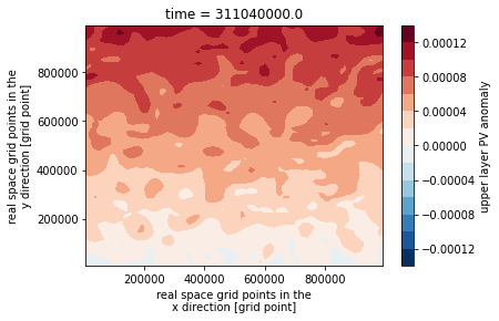
Visualize Output
Let’s assign a new data variable, q_upper, as the upper layer PV anomaly. We access the PV values in the Dataset as m_ds.q, which has two levels and a corresponding background PV gradient, m_ds.Qy.
[4]:
m_ds['q_upper'] = m_ds.q.isel(lev=0) + m_ds.Qy.isel(lev=0)*m_ds.y
m_ds['q_upper'].attrs = {'long_name': 'upper layer PV anomaly'}
m_ds.q_upper.plot.contourf(levels=18, cmap='RdBu_r');
Plot Diagnostics
The model automatically accumulates averages of certain diagnostics. We can find out what diagnostics are available by calling
[5]:
m.describe_diagnostics()
NAME               | DESCRIPTION
--------------------------------------------------------------------------------
APEflux    | spectral flux of available potential energy
APEgen     | total available potential energy generation
APEgenspec | the spectrum of the rate of generation of available potential energy
Dissspec   | Spectral contribution of filter dissipation to total energy
EKE        | mean eddy kinetic energy
EKEdiss    | total energy dissipation by bottom drag
ENSDissspec | Spectral contribution of filter dissipation to barotropic enstrophy
ENSflux    | barotropic enstrophy flux
ENSfrictionspec | the spectrum of the rate of dissipation of barotropic enstrophy due to bottom friction
ENSgenspec | the spectrum of the rate of generation of barotropic enstrophy
Ensspec    | enstrophy spectrum
KEflux     | spectral flux of kinetic energy
KEfrictionspec | total energy dissipation spectrum by bottom drag
KEspec     | kinetic energy spectrum
entspec    | barotropic enstrophy spectrum
paramspec  | Spectral contribution of subgrid parameterization (if present)
paramspec_APEflux | total additional APE flux due to subgrid parameterization
paramspec_KEflux | total additional KE flux due to subgrid parameterization
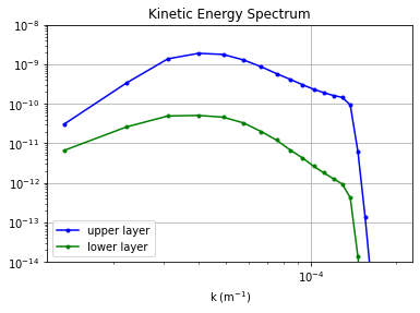
To look at the wavenumber energy spectrum, we plot the KEspec diagnostic. (Note that summing along the l-axis, as in this example, does not give us a true isotropic wavenumber spectrum.)
[6]:
kr, kespec_upper = tools.calc_ispec(m, m_ds.KEspec.isel(lev=0).data)
_, kespec_lower = tools.calc_ispec(m, m_ds.KEspec.isel(lev=1).data)

plt.loglog(kr, kespec_upper, 'b.-', label='upper layer')
plt.loglog(kr, kespec_lower, 'g.-', label='lower layer')
plt.legend(loc='lower left')
plt.ylim([1e-14,1e-8])
plt.xlabel(r'k (m$^{-1}$)'); plt.grid()
plt.title('Kinetic Energy Spectrum');
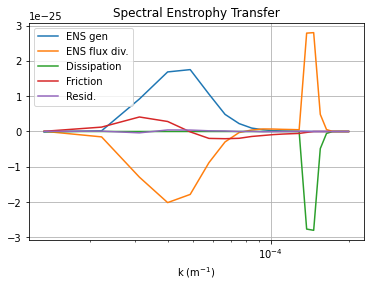
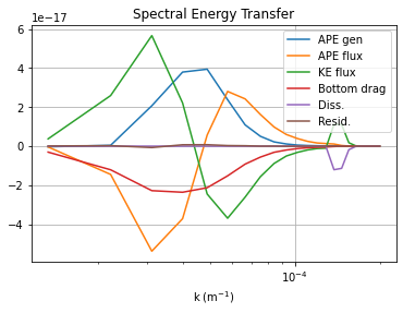
We can also plot the spectral fluxes of energy and enstrophy.
[8]:
kr, APEgenspec = tools.calc_ispec(m, m_ds.APEgenspec.data)
_, APEflux     = tools.calc_ispec(m, m_ds.APEflux.data)
_, KEflux      = tools.calc_ispec(m, m_ds.KEflux.data)
_, KEfrictionspec = tools.calc_ispec(m, m_ds.KEfrictionspec.data)
_, Dissspec    = tools.calc_ispec(m, m_ds.Dissspec.data)

ebud = [ APEgenspec,
         APEflux,
         KEflux,
         KEfrictionspec,
         Dissspec]
ebud.append(-np.vstack(ebud).sum(axis=0))
ebud_labels = ['APE gen','APE flux','KE flux','Bottom drag','Diss.','Resid.']
[plt.semilogx(kr, term) for term in ebud]
plt.legend(ebud_labels, loc='upper right')
plt.xlabel(r'k (m$^{-1}$)'); plt.grid()
plt.title('Spectral Energy Transfer');
[9]:
_, ENSflux    = tools.calc_ispec(m, m_ds.ENSflux.data.squeeze())
_, ENSgenspec = tools.calc_ispec(m, m_ds.ENSgenspec.data.squeeze())
_, ENSfrictionspec = tools.calc_ispec(m, m_ds.ENSfrictionspec.data.squeeze())
_, ENSDissspec = tools.calc_ispec(m, m_ds.ENSDissspec.data.squeeze())

ebud = [ ENSgenspec,
         ENSflux,
         ENSDissspec,
         ENSfrictionspec]
ebud.append(-np.vstack(ebud).sum(axis=0))
ebud_labels = ['ENS gen','ENS flux div.','Dissipation','Friction','Resid.']
[plt.semilogx(kr, term) for term in ebud]
plt.legend(ebud_labels, loc='best')
plt.xlabel(r'k (m$^{-1}$)'); plt.grid()
plt.title('Spectral Enstrophy Transfer');